Scalar Testing (Part Two)
By H. Mark Bowers
In my last column we examined the importance of scalar testing, definitions of various terms, equipment required, and examined waveforms of actual insertion loss and isolation measurements using a spectrum analyzer and tracking generator. If you haven’t read my Part I column, I would recommend that you do so before proceeding with Part II.
Let’s begin with a review of the definitions that we examined in Part I. And we’ll expand on this with an additional test equipment item required in the testing of return loss: the return loss bridge.
Frequency Response: The overall response of a circuit or network displayed as amplitude versus frequency. Frequency response is used to depict how a device operates (gain or loss) as the frequency is varied. The device can be a section of cable, a passive splitter or directional coupler, an amplifier, or even a network segment as in, for instance, system sweeping.
Return Loss: In telecommunications, return loss is the loss of power in the signal returned/reflected by a discontinuity in a transmission line (or optical fiber). This discontinuity can be a mismatch with the terminating load or with a device inserted in the line. It is usually expressed as a ratio in decibels (dB) between the incident (forward) and reflected signals. For more information on return loss, see the Spring 2017 issue of Broadband Library at broadbandlibrary.com/return-loss/
Spectrum Analyzer: A spectrum analyzer measures the magnitude of an input signal versus frequency within the frequency range of the instrument. Its primary use is to measure the power of the spectrum of known and unknown signals. The input signal that a spectrum analyzer measures is usually electrical; however, spectral compositions of other signals, such as acoustic pressure waves and optical light waves, can be measured through the use of an appropriate transducer.
Tracking Generator: See Figure One. A tracking generator operating in conjunction with a spectrum analyzer functions by providing a RF sinusoidal output to the input of the spectrum analyzer. By linking the swept signal of the tracking generator to the spectrum analyzer, the output of the tracking generator tracks (is on the same frequency) the swept input of the analyzer, so that the two units simultaneously track the same frequency, plotting amplitude versus frequency. If the output of the tracking generator is connected directly to the input of the spectrum analyzer, a flat line will be seen, with the amplitude reflecting the output level of the tracking generator less cable and connector losses. If a device under test (DUT), such as a filter, is placed between the output of the tracking generator and the input of the spectrum analyzer, the response of the device under test will alter the level of the tracking generator signal as measured by the spectrum analyzer, with the amplitude versus frequency response of the DUT indicated on the analyzer screen. In this way the response of the DUT will be seen on the analyzer screen.
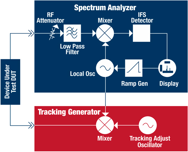
Figure One: Simple block diagram of spectrum analyzer and tracking generator.
Return Loss Bridge: The return loss bridge (RLB), sometimes called a standing wave ratio (SWR) or directional bridge, is typically used to test devices that should show a pass response (indicating high return loss), a reject response (indicating low return loss), or both over a single sweep range. The RLB provides a means of measuring the degree of match or mismatch of the device under test at a particular frequency or frequency range. This is done by measuring the amplitude of the reflected signal (return loss) in decibels compared to a ‘normalized’ 0 dB reference level.
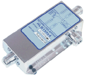
Return loss bridges are typically available in 50 ohm (most common configuration) or 75 ohm impedances, although other specialized impedance values are sometimes encountered. Most return loss bridges have three ports, such as the one shown in Figure Two, and are constructed with a termination built into the device at the appropriate impedance. Some bridges have a fourth port to allow for a high quality external reference termination to be attached. In addition, return loss bridges are designed for a specific bandpass. For example, the 50 ohm return loss bridge shown in Figure Two has a specified frequency range of 5 MHz to 2 GHz, at a return loss of 40 dB or greater across that frequency range.
Figure Two: Typical return loss bridge.
In actuality, there are two insertion losses associated with a RLB: the loss between the source and DUT port, and the loss between the DUT and reflected port. The manufacturer’s specifications may show these insertion loss values separately, or may combine the two losses into a single loss value between the source and reflected ports. In Figure Two, if the DUT port is left open (or shorted), the difference in decibels between the signal applied to the source port and the signal level measured at the reflected port is the insertion loss between the source and reflected ports. The directivity of the bridge is a measure of the quality of the bridge. The directivity of the bridge should be better than the return loss range that you expect to measure in a particular test application. For example, don’t expect to accurately measure return loss values of 50 dB or greater if the directivity of the bridge is rated at 40 dB.
I also mentioned in Part I that the tracking generator and/or return loss bridge can be housed in separate units from the spectrum analyzer, or one or both can be purchased as internal options to the spectrum analyzer. If you plan to acquire these instruments, I would highly recommend that you purchase them as internal analyzer options if possible. When housed internally, space is saved, portability is maintained, quality is preserved, and the appropriate setup and testing routines are simplified.
Finally, I mentioned at the conclusion to Part I that many, if not most, modern spectrum analyzers that provide these measurements are only available with a 50 ohm characteristic impedance. This begs the question “How does one properly test with 50 ohm equipment in the HFC network where the characteristic impedance is 75 ohms?” The solution to this problem comes with the use of one or several minimum loss pads (MLP). A minimum loss (or matching) pad is used to match one real impedance to another real impedance, so that both source and load see the correct impedance. Minimum loss pads enable measurement of broadband 75 ohm networks such as those found in cable television using 50 ohm test equipment. In theory, a 50 to 75 ohm minimum loss pad has 5.7 dB of insertion loss (in either direction for power measurements), and most modern MLPs of sufficient quality have an insertion loss very close to this theoretical value. While this can introduce a large amount of loss into the test setup, our primary concern when measuring return loss is in properly matching differing impedances so that our measurements are as accurate as possible. Where MLPs are placed and the quantity required depends on the measurement taken and whether one is using an internal versus external sweep generator and return loss bridge. The point for now is that maintaining proper impedance matching when using 50 ohm test equipment in a 75 ohm network is crucial to accurate measurements, and the resulting loss due to the insertion loss of the MLP(s) is generally not problematic.
Now let’s examine some frequency response and return loss measurements. The horizontal axis (frequency) is from 80 MHz to 120 MHz in the frequency response measurement (Screenshot One), and from 1 MHz to 3 GHz in all return loss measurements (Screenshot(s) Two through Four).
Screenshot One illustrates the frequency response of a four-section notch filter. The third notch (at marker M1) is at 105.8 MHz, with a notch value of -56.6 dB. Worst case insertion loss for the filter is 5.4 dB as measured at marker M2.
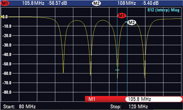
Screenshot One: Frequency response of a four-section notch filter
Screenshot Two (following image) illustrates return loss at the input to a 1 GHz two-way splitter with both output ports properly terminated. Return loss values range from 28 to 30 dB (disregarding some higher return loss spikes at discrete frequencies; return loss values technically are positive values in most cases, although some test equipment incorrectly shows negative numbers) as measured from 1 MHz to 1 GHz. Remember that higher return loss values are what is desired, as this indicates less signal power reflected (back) from the input port of the two-way splitter. The return loss values measured up to 1 GHz are acceptable; but beyond 1 GHz they decrease rapidly such that return loss at 2 GHz is only 3.32 dB!
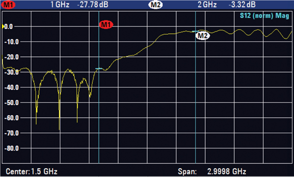
Screenshot Two: Return loss measured at the input port of a two-way splitter
Screenshot Three illustrates return loss measured on the same two-way 1 GHz splitter, only this measurement was taken at one of the two output ports with the input port and remaining output port properly terminated. Return loss below 1 GHz is not quite as good compared to the input port, but is consistent with the manufacturer’s published values. And in similar fashion as compared to the input port measurement (Screenshot Two), return loss above 1 GHz decreases rapidly beyond what is acceptable.
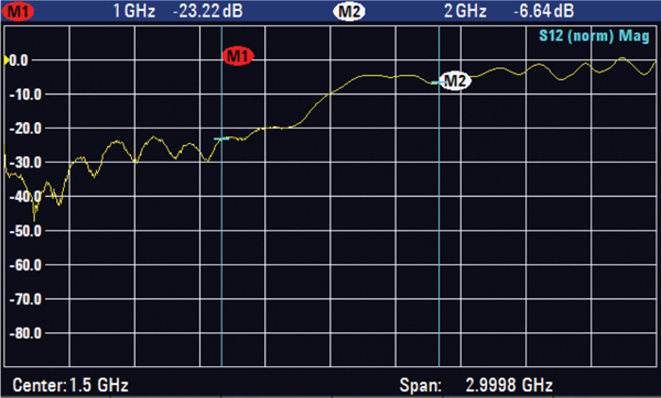
Screenshot Three: Return loss measured at an output port of a two-way splitter
Screenshot Four measures return loss back at the two-way splitter input port, but with an impedance mismatch present at one of the two output ports (with the other port properly terminated). The return loss at 1 GHz is very poor at 8.05 dB.
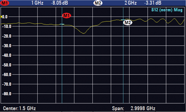
Screenshot Four: Return loss measured at the input port of a two-way splitter, and with a poor impedance match at one of the two output ports
Part II Summary:
- Scalar testing is important from both a theoretical perspective and practical application in the modern HFC plant. For example, based on the measurements performed in Parts I and II of this series, we can reasonably conclude it would be inadvisable to use 1 GHz passives in a 950 to 1450 MHz L-band application based on our insertion loss and return loss measurements.
- Frequency response, isolation, and return loss remain important parameters that should be tested and maintained when critical networks are constructed. Optimal network performance can only be obtained when these parameters are within their proper range.
- In their totality, these measurements illustrate why proper component selection, proper termination of all unused ports, and the use of small-value distributed in-line pads (especially in headend combiner circuitry) are extremely important in achieving and maintaining a network that performs with good frequency response, high isolation between components and network sections, and in the minimizing of reflected signals.
- With a quality spectrum analyzer, tracking generator, and return loss bridge, accurate measurements can be performed. And some newer testing units are quite reasonably priced.
 H. Mark Bowers,
Cablesoft Engineering, Inc.
Mark is VP of Engineering at Cablesoft Engineering, Inc. He has been involved in telephony since 1968 and the cable industry since 1973. His last industry position was VP of Corporate Engineering for Warner Cable Communications in Dublin, OH. Mark’s education includes the U.S. Naval Nuclear Engineering School, and BS and MS Degrees in Management of Technology. Mark is a member of the SCTE, the IEEE, and is a Senior Member and licensed Master Telecommunications Engineer with iNARTE.
Credit: Charts provided by author