Basic HFC AC Design (Part One)
By H. Mark Bowers
Many technicians struggle with AC design, particularly in the area of proper power supply placement and loading. AC design involves concepts and principles that we don’t use in every day system maintenance or operation. HFC design houses and CAD design software now usually handle these complex calculations; however, it remains beneficial to understand overall concepts in order to recognize and properly alleviate powering design issues when they occur.
Because a typical cable system is spread over a wide area, there are unique problems in supplying operating power to its various components. The actives (nodes, amplifiers, etc.) in a cable network are often spaced at considerable distance from each other and may cover a significant geographic area. Each amplifier must be supplied with operating power within an acceptable voltage range. Because integrated circuit RF amplifiers and optics operate at low DC voltages, it would seem ideal to route low-voltage DC within the coaxial cable. This is impractical, however, because of the electrolysis/corrosion problems which can result. Some of the very early coaxial powering systems attempted to utilize DC with less than optimal results; however early telephone coaxial toll systems made successful use of very high-voltage DC powering. This two-part article examines these concepts; then lays out several sample AC designs in order to examine various issues and concerns.
At the most basic level, to determine the voltage drop between system actives along with load voltages at each active, we need the following information:
- The length of each cable segment.
- The DC loop resistance of each cable segment.
- The total current carried in each segment, which ties to the power-current requirements of each active component.
The design is then carried out so that the amplifier(s) most remote from the power supply will always have the minimum required operating voltage supplied under worst case conditions. Further, an ideal design would evenly distribute load voltages through the network while striving for the lowest total current load on the power supply. We’ll examine these ideal design concepts in Part Two.
Coaxial Cable DC Loop Resistance
The nominal frequency of AC power in the U.S. is 60 hertz (Hz). At this very low-frequency, there is little differencebetween the DC loop resistance of the cable and the AC impedance measured at 60 Hz. Impedance is the total opposition to current flow in an AC network at a specific frequency and is rarely purely resistive. Most of the resistance in a coaxial cable comes from the center conductor because of its smaller size, but it is customary to specify the total ‘loop resistance’ of the cable. This is the equivalent resistanceof a given length of cable that includes both center conductor and sheath resistance, and is normally specified by the cable manufacturer in ohms per 1000 feet. Loop resistance (per 1000 ft) varies from less than an ohm for 1″+ diameter cable to over 50 ohms for some types of drop wire.
Ohm’s Law and Cable AC Basics
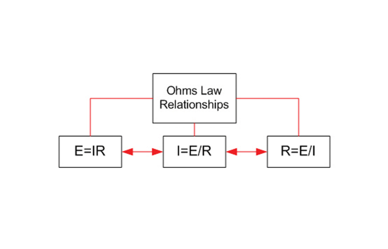
Any discussion on AC powering in cable systems should begin with Ohm’s law. Ohm’s law can be defined by stating — given the three basic electrical quantities of voltage (V), current (I), and resistance (R) — current flow in amperes is directly proportional to total circuit voltage (volts) and inversely proportional to total circuit resistance in ohms (I=V/R). This is one of the most important theorems in electronics because it defines so much about circuit operation. It is simple, and yet forms the foundation for complex theories and circuit analysis. See the top of Diagram One on the following page for the three basic Ohm’s law formulas.
Power Supply Concepts
Cable AC power supplies are normally of the ferroresonant or self-regulating type. This transformer design has proven reliable over many years of use and provides limited surge and voltage variation protection. These transformers use a tank circuit design comprising a resonant winding and capacitor to produce a nearly constant average output voltage under varying current or load conditions. The circuit has a primary on one side of a magnet shunt and a parallel resonant secondary side. The ferroresonant approach is attractive due to its simple design, relying on the saturation characteristics of the tank circuit to absorb variations in input voltage or output load. This circuit also creates a quasi square wave output waveform which provides additional benefits:
- It limits peakvoltage, which assists operators in compliance with local and national codes that limit the peak voltage allowed in communication systems.
- It provides for a more efficient transfer of power from the source to the load.
Power Inserter Considerations
There are three basic considerations involved in coupling a 60 Hz, 60 or 87 VAC supply voltage/current onto a coaxial cable that carries RF signals:
- The RF signals on the coaxial cable should not be shorted by the low impedance power supply transformer secondary windings.
- Noise and other interference that may be present in the electric utility secondary system should not be coupled into the cable system.
- The design of the coupling device should not cause adverse reflections (impedance mismatch) in the 75 ohm impedance HFC plant.
The device that accomplishes this is the power inserter and it meets all these criteria. It is typically housed in an outdoor splitter/directional coupler type case, but may be built into the AC power supply itself.
Amplifier (System Active) Power and Current Ratings
There are two basic power pack designs (converts incoming AC to DC voltages for amplifier/node circuit use) that have been employed over the years. Older equipment (pre-1980s) typically employed linear modepower supplies, which consume a constant currentover a given voltage range. However, most power packs (any modern internal power supply) designed since the 1980s are switch-modedesign. How the two designs differ internally is beyond the scope of this article. A switch-mode supply draws constant powerover a specified input voltage range. This means that as the incoming voltage drops the switch-mode supply will increase its current consumption, which creates additional design calculation complexity that we will examine further in Part Two of this series.
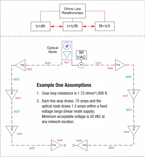
Using the line equipment power ratingwill result in more accurate AC power designs, but accuracy is highly dependent on the computational technique used during the design. If you have access to an AC calculation program that supports a constant power calculation method, I recommend its use. My own (Cablesoft Engineering) AC design program is ancient (coded in the early 1980s in compiled BASIC) but very accurate. As you’ll see in Diagrams Two through Four on the following page and further in Part Two, the user interface is not fancy but calculated results are highly accurate.
Basic AC Network Design Calculations
The maximum voltage in our design is established by our AC power supply choice and NESC/NEC/local code limitations, while the minimum voltage is established by system active requirements.
Referring to Diagram One, if a certain level of energy is supplied to an energy absorbing device, a portion of the energy will be absorbed and dissipated in some fashion (or in some instances stored for later use). Electrically, this energy is known as power and is measured in watts. From Ohm’s law we see that for a fixed current flow and a specific value of resistance, there will be a voltage drop across this resistance (V=IR). The power consumed by a purely resistive device equals the current (amperes) times the voltage drop (volts) across the resistance in ohms (P=IV). In an HFC network, active devices and cable sections create voltage drops and thus consume power. In a resistive network, the sum of all voltage drops (active and cable) equals the supply voltage. In reality, this condition only occurs (all power absorbed by the load) when the load is purely resistive (has no inductive or capacitive components). A cable distribution network is not purely resistive; however, for low-frequency AC design purposes we will assume that it is.
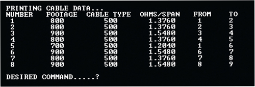
In the remainder of Part One we’ll examine basic calculations assuming all system actives are linear modeand therefore draw a constant current over a given voltage range. In this situation, the calculations are relatively straightforward. Examining the network diagram in Diagram One, any section of cable carrying current will have some voltage drop per unit of length. As current increases, the voltage drop increases. Diagram Two illustrates the calculated total resistance of each span between ‘nodal numbers’ located in the sample layout in Diagram One. The term nodal numberis meant to apply to various points in our design layout, and does not refer to an optical node. See Diagram One for nodal numbers (Nd1, Nd2, etc.). The FROM — TO columns refer to those nodal locations in Diagram One. You can easily confirm the ‘loop resistance’ calculations in Diagram Two. For example, the distance from nodal point #1 to #2 in Diagram One is 800 ft. Since loop resistance is 1.72 ohms per 1,000 ft, [800/1000] x 1.72 = 1.376 ohms as shown in the first numeric row in Diagram Two.
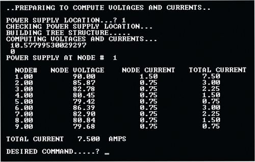
Since we assume a constant current per active, the network voltages and currents behave exactly as we would expect, and total power supply loading remains constant no matter where we place the power supply. For calculation purposes I specified that the minimum voltage at any network point must be ≥50 VAC. The Node Voltage column in Diagram Three shows that our lowest network voltage is at nodal point #5 and is 79.42 VAC so we achieve our basic design parameters.
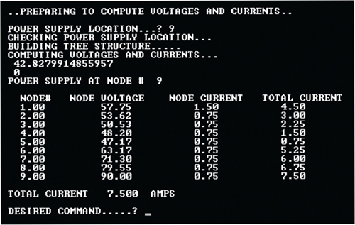
The calculations in Diagram Four illustrate results if we move the power supply to nodal point #9, a network extremity (worst case condition). Total power supply loading remains at 7.5 amperes, but note that voltages at nodal points #3, 4 and 5 are at or below our 50 VAC limit!
This all appears rather well behaved but something is wrong. Moving the power supply location does affect total current loading, so these assumptions don’t reflect a ‘real world’ HFC network. Remember that with switch-mode power supplies current increases as the voltage decreases (constant power). In order to make accurate calculations in this situation, we need an ‘iterative’ calculation process that will take this into account. That will be our starting point in Part Two, where we will also examine ‘odd’ network behavior that can occur when switch-mode designs are not properly accomplished.
 H. Mark Bowers,
Cablesoft Engineering, Inc.
Mark is VP of Engineering at Cablesoft Engineering, Inc. He has been involved in telephony since 1968 and the cable industry since 1973. His last industry position was VP of Corporate Engineering for Warner Cable Communications in Dublin, OH. Mark’s education includes the U.S. Naval Nuclear Engineering School, and BS and MS Degrees in Management of Technology. Mark is a member of the SCTE, the IEEE, and is a Senior Member and licensed Master Telecommunications Engineer with iNARTE.
Credit: Charts provided by author