Scalar Measurements with a Broadband Noise Generator
By H. Mark Bowers
In a previous two-part article (Summer & Fall 2017 Testing in Progress columns, www.broadbandlibrary.com) I demonstrated how to conduct accurate ‘scalar’ measurements using a spectrum analyzer with an integrated tracking generator. Tracking generators, especially those built into newer spectrum analyzers, provide for very accurate methods (± 1/10th dB typical) by which one can measure frequency response and isolation. And with the addition of an RF return loss bridge, return loss measurements can be made with equal precision. Please review my previous Broadband Library articles at https://tinyurl.com/ychaeacm for detail.
But what if your present spectrum analyzer doesn’t have a tracking generator, you can’t afford to purchase one that does, and a measurement accuracy of around ± 1 dB is acceptable? Broadband noise generators offer a viable alternative to the tracking generator approach. A fairly flat RF output response noise generator can be purchased for several hundred dollars and can be paired with most spectrum analyzers. Your analyzer needs to have a good trace averaging routine, and a sample RF detector mode if possible. A sample detector mode displays, for each trace-point, the transient level corresponding to the central time point of the corresponding time interval. If your analyzer doesn’t have this RF detector mode, you can use peak detector mode instead.
Before purchase, noise generator features to consider are RF noise output flatness, RF average output power, and overall frequency range. Portability and physical size should also be considered. The unit employed for these measurements is about the size of a pack of cigarettes, runs on a 9V battery, has an RF average output power of 0.5 dBmV (measured at 1 MHz resolution bandwidth [RBW]), a (Gaussian) noise frequency range from 5 MHz to 2,150 MHz, and is flat to within ± 1 dB across that entire frequency range. And flatness improves as smaller spectral portions are measured: 164 MHz to 216 MHz, for example, is flat to ± 0.4 dB. While the noise method is not as precise as a tracking generator and lacks automated ‘normalization’ routines to account for cable and connector response, it nonetheless offers reasonably accurate measurements as you’ll soon discover. Now let’s examine some typical measurements that can be performed.
Figure 1 illustrates the overall response of my noise generator output from 10 MHz to 1.5 GHz using a direct adapter (F-71). As already mentioned, the range of this generator extends to 2.15 GHz, however, I’ve chosen a spectrum analyzer that only measures to 1.5 GHz because of its versatile vertical and horizontal marker system. Figure 1 shows that the noise RF output for this spectral portion is flat to the same specifications listed in the preceding paragraph. For component testing I’m using two 6 ft Series RG-59 jumpers that can introduce some tilt depending on the frequency measurement range. When using a noise generator, we’ll have to be satisfied with an overall measurement accuracy of ± 1 db at best, so I will ignore any slope introduced and assume a flat RF output of 0 dBmV average power level for our measurements unless otherwise noted. Also note that the blue trace is an average of 50 traces using a sample detector. This helps to flatten our trace to obtain optimal accuracy with this method.
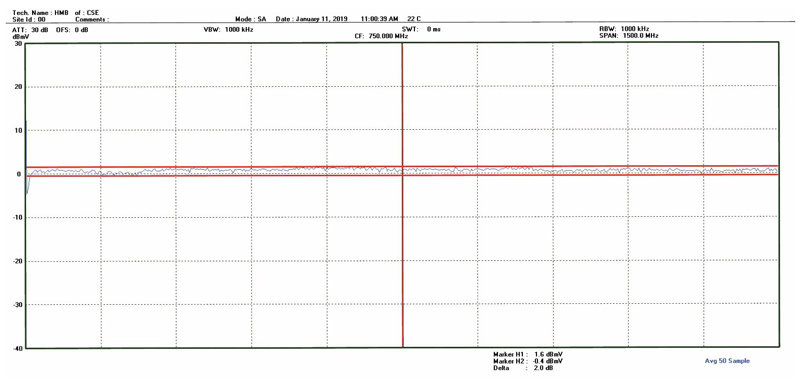
Figure 1. Response of noise generator output – 10 MHz to 1.5 GHz
In Figure 2, I’m feeding the noise generator output into one of the two output legs of a standard quality home installation 1 GHz 2-way splitter. The input port is terminated, and the other output port is connected to the spectrum analyzer input. This provides for a fairly accurate measurement of the isolation between output ports at any frequency. I’ve placed a horizontal marker at 0 dBmV (the average RF noise power generator output), and I’ve placed vertical markers at 50 MHz and 1 GHz, the downstream spectral range that I want to measure. Several observations can be made with this screen capture.
- Isolation is much better at lower frequencies than in the upper spectrum, with the isolation at 50 MHz approximately 35 dB while it has dropped to 22 dB at 1 GHz.
- As we increase in frequency beyond 1 GHz (the upper frequency design limit of this splitter), isolation continues to worsen. By 1.5 GHz isolation is estimated at 15 dB.
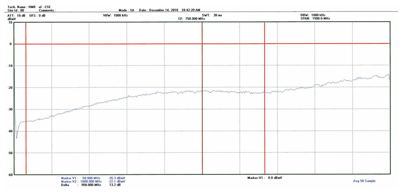
Figure 2. Isolation between 1 GHz splitter output ports — input port terminated
Figure 3 illustrates greatly reduced output port isolation when the splitter input is poorly terminated. Almost all isolation is gone, and the trace takes on a rippled appearance in the presence of standing waves (reflected power). The best-case isolation appears to be 9 dB, but that’s only at {the} specific low-points of each standing wave. Average isolation is around 7.5 dB.
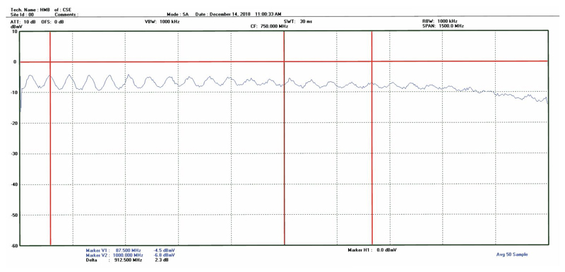
Figure 3. Isolation between 1 GHz splitter output ports — input port poorly terminated
Figure 4 illustrates the response of a filter designed to pass Ch. 7 through Ch. 13 frequencies. The lower frequency vertical marker is centered in the midpoint of the bandpass region. Rejection of adjacent frequencies close to the filter bandpass response is almost 50 dB; however, note that in the 750 MHz to 900 MHz range isolation is reduced to below 30 dB at certain frequencies. Also note that insertion loss through the desired region (174 MHz to 216 MHz) increases with frequency. While insertion loss at Ch. 7 is close to 0 dB, at Ch. 13 it’s approximately 4 dB.
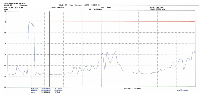
Figure 4. Response of Ch. 7 through Ch. 13 bandpass filter
Figure 5 illustrates the bandpass of a headend diplex filter, with noise injected at the common port and the spectrum analyzer input connected to the low-pass port (5 MHz to 42 MHz). The high-pass port (48 MHz to 1,000 MHz) is terminated. Note also that I’ve zoomed in to show the response from 5 MHz to 205 MHz only, and have reduced RBW from 1 MHz (used in my other measurements) to 300 kHz. The average RF output noise power of the generator now measures at -4 dBmV. Remember that average RF noise power level is dependent on the bandwidth at which it is measured. For example, if the RBW on my analyzer is increased to 6 MHz, the RF average output power level of the noise generator measures close to +10 dBmV!
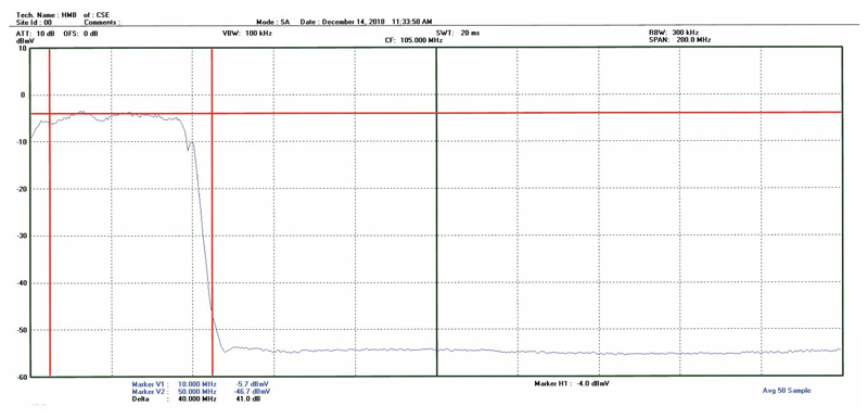
Figure 5. 5 to 42 MHz Band Response of a Standard Headend Diplex Filter with the High Side Terminated
Figure 5’s response shows an insertion loss of 1.5 dB at 10 MHz, while at 50 MHz (well past the low-high crossover point of the diplex filter) the rejection (isolation) of the high-pass region is approximately 43 dB and increases beyond that. At 65 MHz the high-side isolation is greater than 50 dB!
In Figure 6, our final waveform, we’re measuring the ‘through’ response of a 4-way L-band splitter, with an optimized frequency response from 950 MHz to 1,450 MHz. The insertion loss at 950 MHz is 7.4 dB, and 8.3 dB at 1,450 MHz. Note that the response below approximately 750 MHz is poor, with standing waves present even though all unused ports are terminated. This illustrates why you should never use an L-band splitter elsewhere in your plant or headend combining network; L-band splitter response is optimized for the L-band frequency range only.
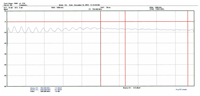
Figure 6. Through response of L-band 4-way splitter with unused legs terminated
Conclusion
My hope is that this article has piqued your interest in cable television scalar related measurements that can be performed with a portable broadband noise source. In actuality, there are more measurements that can be performed beyond isolation and frequency response. Noise generators can be used as a reference source to measure system level noise figure, signal simulation, as a {noise} source for bit error ratio (BER) testing, and for evaluating analog and DOCSIS HFC system dynamic range.
If you’d like more information about the noise generator used to perform these measurements, feel free to contact me at the email address provided below.
 H. Mark Bowers,
Cablesoft Engineering, Inc.
Mark is VP of Engineering at Cablesoft Engineering, Inc. He has been involved in telephony since 1968 and the cable industry since 1973. His last industry position was VP of Corporate Engineering for Warner Cable Communications in Dublin, OH. Mark’s education includes the U.S. Naval Nuclear Engineering School, and BS and MS Degrees in Management of Technology. Mark is a member of the SCTE, the IEEE, and is a Senior Member and licensed Master Telecommunications Engineer with iNARTE.
Credit: Charts provided by author