How Adaptive Equalization Works
By Ron Hranac
Digital communications systems are designed to transmit high-speed data through band-limited channels—for example, 6 MHz-wide downstream channels or 6.4 MHz-wide upstream channels, which are susceptible to various distortions. The presence of distortion in the channel results in something called inter-symbol interference (ISI), which can cause data transmission errors. One way to compensate for or reduce ISI is to incorporate an equalizer in the receiver or transmitter. If the channel characteristics are known and don’t change over time, fixed-value equalizers can be used. However, in a typical cable network the signal path between the headend and each cable modem (or digital set-top box) is unique, so a one-size-fits-all fixed equalizer is impractical. Furthermore, distortions causing ISI can change over time, so the equalizer must somehow be adjustable to compensate for changes in channel conditions. Adaptive equalizers are most often used for this purpose. How do they work and how does adaptive equalization relate to PNM? Read on to find out.
Let’s first look at the concept of equalization from the perspective of a cable distribution network (refer to Figure 1). As you know, in a given length of coaxial cable higher frequencies are attenuated more than lower frequencies. For instance, if the all downstream signals in the, say, 50 MHz to 870 MHz spectrum have the same amplitude at the output of an amplifier, we say the overall frequency response—technically speaking, amplitude (or magnitude)-versus-frequency—is flat. By the time that flat group of signals passes through coax to the next amplifier, it will be tilted because of greater attenuation at higher frequencies than at lower frequencies. In order to get the tilted spectrum flat again, we have to install a fixed-value plug-in equalizer at the second amp. The equalizer is a small passive circuit that has the opposite amplitude-versus-frequency response of the length of coaxial cable preceding the amp. The equalizer is in effect a broadband filter that cancels the tilted response in the operating bandwidth, resulting in a flat amplitude-versus-frequency spectrum at the second amp’s internal gain stages.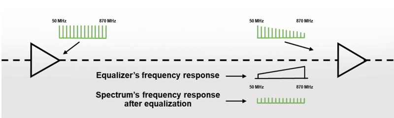
Figure 1. Equalization in the coaxial distribution network
Adaptive equalization performs a function similar to that of a cable amplifier’s fixed-value plug-in equalizer. Rather than equalizing the entire downstream or upstream RF spectrum, it deals with just a single channel. Adaptive means the equalizer can change its characteristics as channel conditions change.
An adaptive equalizer is a digital circuit that compensates for a digital signal’s in-channel complex frequency response impairments. The cable industry has long used the term frequency response to describe amplitude (or magnitude)-versus-frequency—that is, what is seen on the display of test equipment used to sweep outside plant. True frequency response is a complex entity that has two components: amplitude-versus-frequency, and phase-versus-frequency. An adaptive equalizer can compensate for in-channel amplitude- and phase-versus-frequency impairments.
Adaptive equalizers use sophisticated algorithms to derive coefficients for an equalizer solution “on the fly”—in effect creating a digital filter with essentially the opposite complex frequency response of the impaired channel. Because the adaptive equalizer’s complex frequency response is essentially a mirror image of the impaired channel’s complex frequency response, the equalizer cancels out most or all of the degraded in-channel frequency response that is affecting the digital signal—within the limits of the adaptive equalizer’s capabilities, of course. (It’s important to note that at high signal-to-noise ratio or ES/N0 the adaptive equalizer will synthesize the opposite response of the channel. At lower SNR doing so would cause noise enhancement, so a compromise solution is derived.)
If the in-channel impairment suddenly changes or goes away, the adaptive equalizer will distort the signal, until new equalizer coefficients for the current channel conditions are derived and the equalizer’s operation updated. Thankfully, this adaptation process is very fast, typically completed in milliseconds.
In order for an adaptive equalizer’s algorithms to begin the process of deriving coefficients that will be used to create a “filter” whose complex frequency response is opposite of the channel’s complex frequency response, the equalizer starts with an adaptation source. The adaptation source can be a transmitted training sequence, or the signal itself.
- Transmitted training sequence: In conventional zero-forcing or minimum mean square error (MSE) equalizers, a known training sequence is transmitted to the receiver for the purpose of initially adjusting equalizer coefficients. In the DOCSIS® upstream pre-equalization process, data transmissions from all cable modems include a preamble at the beginning of each burst. The preamble is used as a training signal for the cable modem termination system’s (CMTS’s) upstream adaptive equalizer.
- The signal itself: Equalizers that do not rely upon transmitted training sequences for the initial adjustment of the coefficients are called self-recovering or blind equalizers. The adaptive equalizer in the downstream receiver of a DOCSIS cable modem (or a digital set-top) is a blind equalizer. In the case of cable modems, DOCSIS does not specify a training sequence in the downstream signal.
As mentioned previously, algorithms are used to automatically adjust equalizer coefficients to achieve optimum performance, and to rapidly adapt to changing channel characteristics. General criteria for defining optimum performance include minimizing peak distortion at the equalizer output, or minimizing the MSE at the equalizer output. In other words, the algorithm adjusts equalizer coefficients on the fly to converge on a solution that best reduces, say, MSE, which improves receive modulation error ratio (RxMER).
An important parameter in an adaptive equalizer is its span, which is directly related to the maximum amount of time delay in a micro-reflection that can be compensated for. If the channel response contains a reflection (caused by an impedance mismatch) that has a longer time delay than the span of the equalizer, the equalizer can’t compensate for that reflection.
Figure 2 illustrates a block diagram of a generic adaptive equalizer. The top row with boxes labeled Z-1 can be thought of as a tapped delay line. Each box marked Z-1 is a delay element, with the amount of time delay per “box” equal to the reciprocal of the symbol rate in a T-spaced equalizer. A delay element is often called a tap, but a tap also can be considered the combination of a delay element, the point where some of the signal is “tapped” off, and a multiplier. The boxes labeled b-2, b-1, b0, etc., are multipliers with equalization coefficients that set the gain for each tap. The algorithm adjusts the equalization coefficients that set the gain for each multiplier. The circles marked Σ are summing or combining circuits.
One tap is called the main tap (highlighted in red in Figure 2). The main tap has a gain of 1, and passes the input signal at its original amplitude. Other taps represent either the “past” or “future” relative to the main tap, and vary the amplitudes of the respective signals passing through them as required.
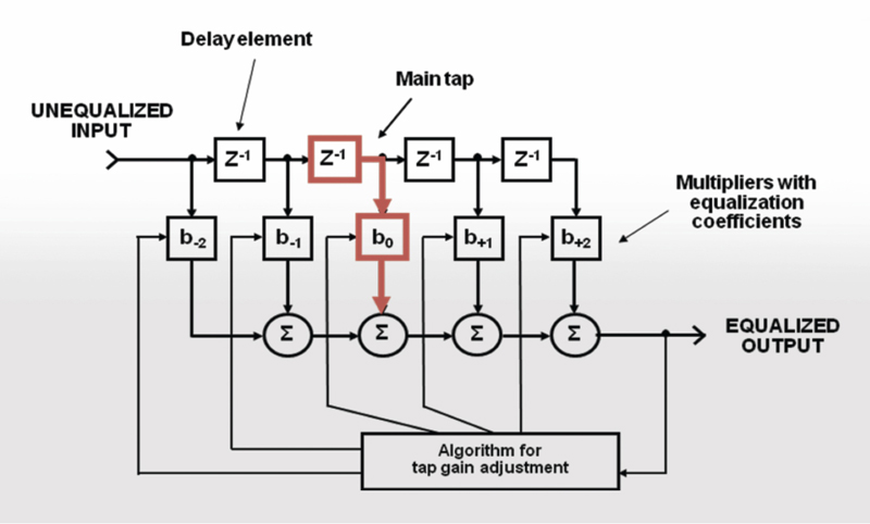
Figure 2. Block diagram of a generic adaptive equalizer
An analog equivalent of what’s going on here is something like the following: Each of the Z-1 delay elements in Figure 2’s example is equivalent to about 167 feet of “lossless” coaxial cable (it takes RF about 1.17 ns to travel through a foot of hardline coax, so 167 feet of coax delays the signal by approximately 195 ns). Each “bn” multiplier is equivalent to a variable attenuator. Attenuator b0 is adjusted for no attenuation (unity gain), and each of the others is adjusted by an amount determined by the algorithm and resulting coefficients. Each of the Σ summing circuits can be thought of as backwards two-way splitters functioning as combiners, except that these, too, are assumed to be “lossless” for this example. Keep in mind that this analog equivalent is just that—an equivalent. A real-world adaptive equalizer (or pre-equalizer) is actually a digital circuit, but you can think of its operation as functionally similar to an analog circuit that combines different amplitudes and phases of an input waveform to achieve a desired output waveform.
As mentioned earlier, a cable modem uses a blind adaptive equalizer in the device’s downstream QAM receiver; the equalization is done after the signal is received by the modem. DOCSIS 1.1 and later cable modems are capable of equalizing—or more accurately, pre-equalizing—the upstream signal prior to transmission. DOCSIS 1.1 supports 8-tap upstream pre-equalization, and DOCSIS 2.0 and 3.0 support 24-tap upstream pre-equalization.
You might be inclined to ask, “Why pre-equalize in the modem?” One reason is because the path between each cable modem and the CMTS is unique. Perhaps more important, pre-equalization allows most of the adaptive equalization to be done by the modem before upstream transmission, rather than relying upon the CMTS to do all of the work.
Pre-equalization in the modem sounds like a good idea, but a cable modem has no way of knowing the condition of the channel between its upstream transmitter output and the CMTS’s input. The modem can’t “see” the channel through which the upstream digitally modulated signal is transmitted. So how can a cable modem correctly pre-equalize a transmitted upstream signal?
Here’s a high-level overview of how upstream pre-equalization works. The cable modem transmits (among other things) station maintenance bursts to the CMTS, which uses the preamble of the unequalized (RNG-REQ) station maintenance message as a “training signal” for the equalization process. The CMTS’s upstream burst receiver includes an adaptive equalizer that derives coefficients based on the channel impairment(s) affecting the received signal.
After converging on a solution for that modem’s received signal, the CMTS transmits the derived equalizer coefficients to the modem in a RNG-RSP MAC message. The cable modem uses those coefficients in its upstream adaptive equalizer to pre-equalize or pre-distort the transmitted signal, so that when it is received by the CMTS it will, in theory, be unimpaired.
Adaptive Equalization and PNM
How does all of this relate to PNM? In-channel frequency response (ICFR) and other parameters can be derived from pre-equalization coefficients, making it possible to determine the extent of an upstream channel’s impairment. Modems that “see” more or less the same ICFR can be identified and grouped, and that information overlaid on system maps to help locate the impairment causing the problem! Adaptive pre-equalization was the basis for early PNM tools, and remains an important part of the latest tools.
A big thanks to Broadcom’s Bruce Currivan (now retired) and CableLabs’ Tom Williams, for the time they took several years ago to explain to yours truly some of the basics of adaptive equalization.
 Ron Hranac
Technical Marketing Engineer,
Cisco Systems
rhranacj@cisco.com
Ron Hranac, a 46-year veteran of the cable industry, is TME for Cisco’s Cable Access Business Unit. A Fellow Member of SCTE and co-founder and Associate Board Member of the organization’s Rocky Mountain Chapter, Ron was inducted into the Society’s Hall of Fame in 2010, is a co-recipient of the Chairman’s Award, an SCTE Member of the Year, and is a member of the Cable TV Pioneers Class of ’97. He received the Society’s Excellence in Standards award at Cable-Tec Expo 2016. He has published hundreds of articles and papers, and has been a speaker at numerous international, national, regional, and local conferences and seminars.