The Untapped Capacity of Coaxial Cable
By Ron Hranac
The cable industry has for many years been migrating optical fiber technology closer to the end user. Ever since the introduction of what we now call hybrid fiber/coax (HFC) architectures, the end goal has arguably been fiber-to-the-home (FTTH). Indeed, many operators already have some FTTH deployments, although they are for the most part single digit percentages of total plant. FTTH often makes sense in new build or greenfield applications, but it’s still pretty costly to rip out an existing HFC network and replace it completely with fiber. That said, why the interest in FTTH? In a word, capacity.
Lawrence Lockwood’s article “Optical bandwidth” in the June 1990 issue of Communications Technology magazine described the capacity of single mode fiber as about 20 THz. That works out to the equivalent of something like 3.3 million 6 MHz-wide channel slots. That kind of capacity surely spells doom for coaxial cable, right? Not so fast. First, the full capacity of optical fiber won’t be utilized for a long, long time. The limitation isn’t the glass itself, but rather the electronics connected to the ends of the fiber. Still, expect to see service providers continue to take advantage of all the optical fiber capacity they can.
Today’s coaxial cable
What about coaxial cable? The industry is moving to 1.8 GHz networks, but that isn’t the limit to what HFC architectures have the potential to support. Coaxial cable still has a fair amount of untapped capacity that can carry our networks well into the future. How much? More than you might think.
Modern hardline and drop cables are spec’d to 3 GHz. That’s a capacity of almost 500 6 MHz-wide channel slots between 5 MHz and 3 GHz. Not bad.
Is 3 GHz as high as we can go with coax? The answer is a resounding “it depends.” There are both practical and theoretical limitations. Let’s start with the theoretical limitations. For this discussion I’m focusing on just the coaxial cable itself, not actives, passives, connectors, etc.
Coaxial cable TE mode cutoff frequency
The desired mode of propagation in coaxial cable is known as the transverse electromagnetic (TEM) mode. Higher modes such as transverse electric (TE) are undesirable, in part because the electric and magnetic fields are non-uniform, and the interactions between the fundamental TEM mode and higher modes can cause unwanted problems. The first higher order mode, called TE11, can propagate above the TE mode cutoff frequency fc. Ideally, the maximum operating frequency in coaxial cable should not exceed fc, such that only TEM mode is supported. The following formula can be used to calculate fc for TE11 mode in coaxial cable.
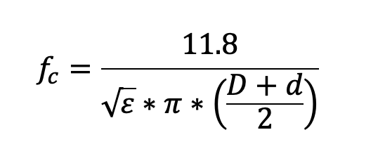
where
fc is the TE11 mode cutoff frequency in gigahertz (GHz)
ε is the cable’s dielectric constant
D is the inner diameter of the cable’s shield, in inches
d is the outer diameter of the cable’s center conductor, in inches
The cable’s center conductor diameter and shield inside diameter (or dielectric outside diameter), illustrated in Figure 1, can be found in coaxial cable manufacturers’ published specifications. The dielectric constant usually isn’t a published value, but can be calculated from the velocity factor (VF), the decimal form of velocity of propagation, using the formula ε = 1/VF2. For instance, if VF is 0.87, the dielectric constant is 1/0.872 = 1.32.
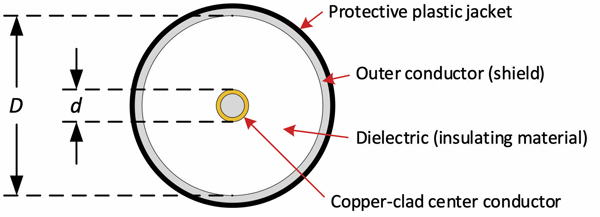
Figure 1. Coaxial cable dimensions of interest, D and d, for calculating fc.
Example: What is fc for .500 hardline foam dielectric coaxial cable, assuming the center conductor diameter d is 0.109 inch, the inner diameter of the shield D is 0.452 inch, and the dielectric constant is 1.32?
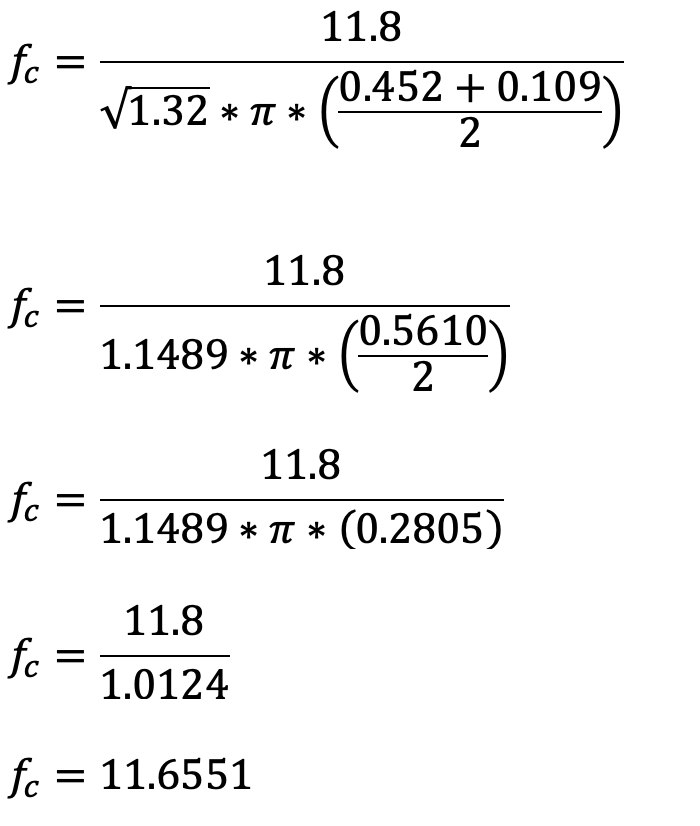
Answer: The TE11 mode cutoff frequency fc for .500 hardline coax is about 11.66 GHz.
Crunching the numbers for a couple other cable sizes gives us a calculated fc for .750 hardline coaxial cable (D = 0.680 inch, d = 0.167 inch, and ε = 1.32) of about 7.7 GHz, and fc for Series 6 drop cable (D = 0.18 inch, d = 0.04 inch, and ε = 1.38) of about 29.06 GHz. The theoretical capacity for each of the cable sizes just discussed is summarized in Table 1.
Perhaps somewhat surprisingly, fc is higher for smaller diameter cables than it is for larger cables. While smaller diameter cables have a higher fc and a theoretically greater capacity, they also have a higher attenuation per unit length than larger diameter cables. That takes us from theoretical limitations to practical limitations.
Attenuation: the gotcha
While calculated fc suggests we can use some pretty high frequencies in coaxial cable, one major gotcha is the cable’s attenuation at those higher frequencies. I don’t think there is any practical way to use Series 6 drop cable up to 29 GHz. The attenuation, which I calculated to be a bit more than 35 dB/100 ft. at that frequency, would almost certainly be a show stopper for any length beyond more than a few feet.
Instead, let’s just go an octave above today’s 3 GHz upper end for published cable specs, to 6 GHz. That accommodates the use of 0.750 hardline, which has a calculated fc of 7.7 GHz. Table 2 shows the calculated approximate losses (using the square root of frequency method, see sidebar) at 6 GHz for the three previously mentioned cable types. The number of full 6 MHz-wide channel slots from 5 MHz to 6 GHz works out to 999.
Data throughput
What kind of data speeds could be supported in nearly 6 GHz of RF spectrum? Let’s start by splitting that spectrum roughly in half, with the dividing line between the upstream and downstream at 3 GHz. The 5 MHz to 3 GHz upstream spectrum could carry 31 full orthogonal frequency division multiple access (OFDMA) channels that are each 96 MHz wide, and the 3 GHz to 6 GHz downstream spectrum could carry 15 full orthogonal frequency division multiplexing (OFDM) channels, each 192 MHz wide. Assuming the use of 4096-QAM, each 96 MHz-wide upstream OFDMA channel can provide about 0.94 Gbps with 25 kHz subcarrier spacing, for a total throughput of about 29 Gbps. In the downstream, each 192 MHz-wide OFDM channel can provide roughly 1.89 Gbps with 25 kHz subcarrier spacing, for a total throughput of about 28 Gbps.
To keep things simple, I’ve left out RF bandwidth lost to a diplex filter transition region. If the electronics don’t need diplex filters (that kind of technology already exists), all the better. I think it’s safe to say a 6 GHz network could easily support upwards of 25 Gbps symmetrical data speeds, even more if higher modulation orders are used (remember, DOCSIS optionally supports 8192-QAM and 16384-QAM).
Wrapping up
At some point in the future FTTH will be ubiquitous. I’ll defer to the finance folks to sort out when it makes sense dollar-wise to jump to all-fiber operation. In the meantime, HFC networks will be here for the foreseeable future, taking advantage of the combined capacities of optical fiber and coaxial cable technology. 1.8 GHz networks are just around the corner, and the use of frequencies as high as 3 GHz are on the horizon. We don’t have to stop there. The untapped capacity of coaxial cable might be able to accommodate operation to at least 6 GHz, maybe more. Of course, hardline and drop cable would have to be tested at frequencies above 3 GHz, confirming attenuation performance and parameters such as structural return loss (SRL). Actives, passives, connectors, and other components would need to be designed for >3 GHz operation, too. Whether a practical future upper frequency limit is 6 GHz or something else remains to be determined, but the bottom line is we haven’t yet reached a capacity stopping point for coaxial cable.
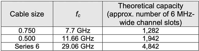
Table 1. Theoretical RF capacity for 0.750, 0.500, and Series 6 coaxial cables.
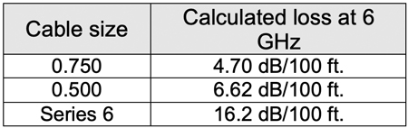
Table 2. Calculated cable loss at 6 GHz
Sidebar:
Calculating cable loss with the square root of frequency method
Some of the following is from the operational practice SCTE 270 2021r1, “Mathematics of Cable”:
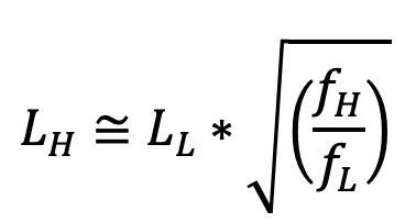
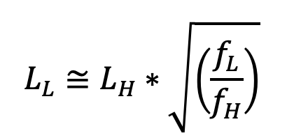
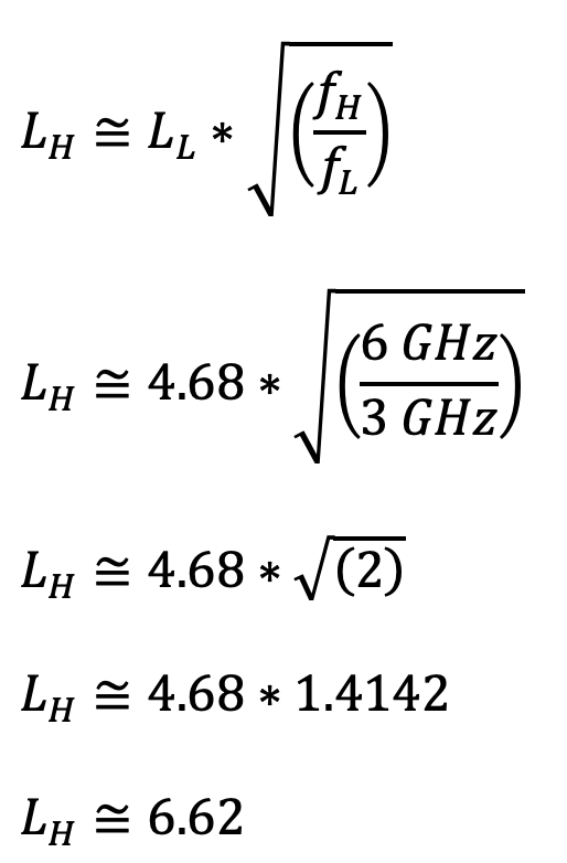
The ratio of coaxial cable attenuation, in decibels, at two frequencies is approximately equal to the square root of the ratio of the two frequencies. From this, one can calculate the approximate loss at one frequency when the loss at another frequency is known, using the following formulas:
where
LH is the approximate loss in decibels at frequency fH
LL is the known loss in decibels at frequency fL
fH is the high frequency of interest
fL is the low frequency of interest
where
LL is the approximate loss in decibels at frequency fL
LH is the known loss in decibels at frequency fH
fL is the low frequency of interest
fH is the high frequency of interest
I used the first formula to calculate the approximate loss per 100 feet at 6 GHz for the three cables in the article. Here’s an example for 0.500 hardline coax. Its published attenuation at 3 GHz is 4.68 dB/100 ft. The approximate loss at 6 GHz is calculated as follows.
 Ron Hranac
Technical Editor,
Broadband Library
rhranac@aol.com
Ron Hranac, a 50 year veteran of the cable industry, has worked on the operator and vendor side during his career. A Fellow Member of SCTE and co-founder and Assistant Board Member of the organization’s Rocky Mountain Chapter, Ron was inducted into the Society’s Hall of Fame in 2010, is a co-recipient of the Chairman’s Award, an SCTE Member of the Year, and is a member of the Cable TV Pioneers Class of ’97. He received the Society’s Excellence in Standards award at Cable-Tec Expo 2016. He was recipient of the European Society for Broadband Professionals’ 2016 Tom Hall Award for Outstanding Services to Broadband Engineering, and was named winner of the 2017 David Hall Award for Best Presentation. He has published hundreds of articles and papers, and has been a speaker at numerous international, national, regional, and local conferences and seminars.
Images provided by author