Scalar Testing (Part ONE)
By H. Mark Bowers
In my last column we examined digital QAM testing requirements under present FCC Part 76 Rules and ANSI/SCTE 40 2003 Requirements. In this column we’ll begin an examination of scalar testing and why it’s important in the HFC network.
When I became involved in cable television in the spring of 1973, the company I joined spent an inordinate amount of time in the training, proper use and application of scalar testing. It was an ever present guiding principle as we constructed headends and built coaxial distribution plant during the exciting years when many communities’ first franchises were issued. Beginning with the downstream combining network, where frequency division multiplexing is employed to combine all signals before driving lasers or the coaxial cable plant; optimal isolation, frequency response, impedance matching, and the minimizing of reflected signals is vitally important to overall performance and signal quality. In the early 1970s, we actually tested every component for all of the these parameters before placing them in the headend or outside plant. Splitters, directional couplers, filters, and modulators and processors were tested separately and then tested again as combiner sections were assembled. All reels of cable and all amplifiers were tested for frequency response and return loss before placement in the plant. Some of this had to do with inconsistent quality as compared to today’s components and equipment; however, I would argue that in network critical applications these are still advisable practices to follow. So why are these concepts and measurements so important, then and now?
In Part I we will examine insertion loss and isolation measurements, while in Part II we’ll examine frequency response and return loss measurements.
Let’s Start with Definitions of the Properties that We will Examine in Parts I and II
Scalar Testing
At its simplest level, scalar refers to a quantity consisting of a single real number used to measure magnitude. This real number can represent power (as in a spectrum analyzer), voltage, or temperature measurements to name just a few. Scalar testing, as applied to the HFC plant, describes a general group of measurements that plot amplitude (usually power) versus frequency. Frequency response, insertion loss, isolation, and return loss all fall within this general category of component or network testing. The common measurement parameters in most scalar test measurements are frequency and amplitude. When a phase component is introduced into the measurement, scalar testing is then correctly called vector testing; since a vector by definition includes both amplitude and phase values. Examples of vector testing are Smith Chart measurements, and constellation diagrams in QAM testing. Vector testing is beyond the scope of this column, but may be examined at another time.
Insertion Loss
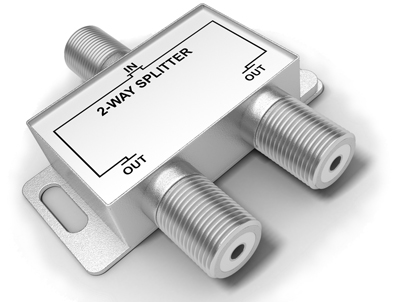
In the case of a two-way splitter, for example, insertion loss is defined as the total loss from the input port to either output port, with the other output port terminated at its proper impedance.
Isolation
The total loss between output ports with the input port properly terminated. Typical values for commercially available splitters are in the 20 to 30 dB range. A directional coupler tap leg possesses directivity; that is, additional isolation from the output port, and this quality of directivity makes the directional coupler highly desirable when combining, extracting, or sampling signals.
Frequency Response
The overall response of a circuit or network displayed as amplitude versus frequency. Frequency response is used to depict how a device operates (gain or loss) as the frequency is varied. The device can be a section of cable, a passive splitter or directional coupler, an amplifier, or even a network segment as in system sweeping.
Return Loss
In telecommunications, return loss is the difference, in decibels (dB), between the power of an incident wave and the power of a reflected wave at an impedance discontinuity in a transmission line (or optical fiber). The discontinuity occurs whenever the impedance of a component or device is not equal to the impedance of the transmission line. (Note: see the column on Return Loss by Ron Hranac in the Spring 2017 Broadband Library at broadbandlibrary.com, and his column in this edition on Decibels.)
Characteristic Impedance (Zc)
The characteristic impedance of coaxial cable (and other cable television components) is nominally 75 ohms, and can be thought of as a purely resistive value (although in practice some reactance also exists, making impedance a complex quantity rather than a scalar quantity) and therefore constant for any unimpaired transmission line. At its simplest level, characteristic impedance is the ratio of voltage to current in a traveling wave within the transmission medium; its value in ohms is also related to the physical dimensions of the transmission line’s center conductor outer diameter and shield’s inner diameter. Also note that the characteristic impedance does not determine the signal attenuation of the transmission line per unit of length. Once the cable industry made the decision to use coaxial cable at a nominal 75 ohms Zc, other components (passives and actives) were manufactured with a corresponding Zc value.
Transmission Line
A transmission line is defined as follows. “In communications engineering, a transmission line is a specialized cable or other ‘structure’ designed to conduct alternating current of radio frequency; that is, currents with a frequency high enough that their wave nature must be taken into account.” By this definition, coaxial cable is a transmission line.
One might reasonably assume that all components manufactured for placement in a 75 ohm headend or plant present a good characteristic impedance at that value, but that would not be the case. Some components present a poor 75 ohm impedance match to the network, with a notch or bandpass filter as examples. And other components have a characteristic impedance (and resulting return loss) that is not as good as one might expect. Distributed padding helps to minimize this problem. By ‘distributed padding’ I mean the placement of small value (loss) in-line resistive pads at various locations in headend combining networks or other network sections. Installation of a pad at the input or output port of a device improves the return loss of that port by twice the value of the pad, and helps to maintain the characteristic impedance overall network closer to the desired 75 ohms value. For those interested in more detail, I authored a separate article on this subject years ago that I can forward upon request.
When passive components are measured, a tracking generator is generally employed, and when return loss is measured a return loss bridge is required as well as a tracking generator. Some spectrum analyzers come with an option for a built in tracking generator, and some analyzers may even include the option for an internal return loss bridge. Absent an analyzer where they are built in, external units are required. For a detailed definition of these devices and their function, check on-line sources such as Wikipedia.
Now Let’s Examine Some Actual Measurements
The following waveforms measure ‘insertion loss’ and ‘isolation’ on a randomly chosen 1 GHz DC-9 directional coupler. All measurements were taken with a high quality spectrum analyzer & tracking generator, with test lead and adaptor losses ‘normalized’ to the 0 dB reference line; therefore the loss values shown on the screen captures are the precise (accuracy better than .1 dB) insertion loss and/or isolation values. The horizontal axis (frequency) is from 10 kHz to 2 GHz in all measurements.
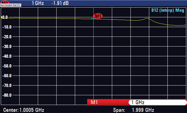
Screenshot One: DC-9 ‘Input’ to ‘Through’ Port
Screenshot One measures insertion loss from coupler ‘input’ to the ‘through’ output leg with the ‘tap’ leg terminated. Insertion loss at 1 GHz is 1.9 dB, which closely matches the manufacturer’s specifications. Also note that the insertion loss from 1 to 2 GHz increases rapidly beyond 1.0 GHz.
Part I Summary
- Scalar testing is important from both a theoretical perspective and practical application in the modern HFC plant. For example, based on these measurements we can conclude it would be inadvisable to use 1 GHz passives in the 950 MHz to 1,450 MHz LNB splitting network!
- Frequency response, isolation and return loss remain important parameters to be tested and maintained when critical networks are constructed. Optimal performance can only be obtained when these parameters are within their proper range.
- With a spectrum analyzer, tracking generator, return loss bridge (next article), very accurate measurements can be made; and some newer testing units are very reasonably priced.
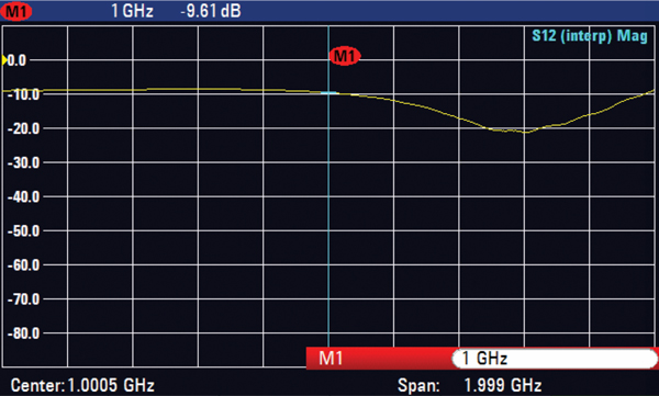
Screenshot Two: DC-9 ‘Input’ to ‘Tap’ Port
Screenshot Two measures insertion loss from coupler ‘input’ to the ‘tap’ output leg with the ‘through’ leg terminated. Insertion loss at 1 GHz is 9.6 dB. Again, note the rapid increase in insertion loss beyond 1 GHz.
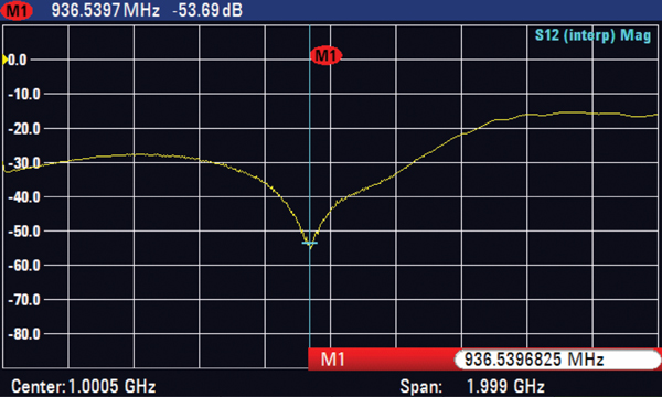
Screenshot Three: DC-9 Output Isolation with ‘Input’ Terminated
Screenshot Three measures isolation from the ‘tap’ to the ‘output’ port (tracking generator signal is injected at the tap leg, isolation is measured at the through leg) with the ‘input’ port terminated. The best-case isolation value is a remarkable 53.7 dB at 936.54 MHz, however average isolation ranges from high 20 dB to low 30 dB values. And note how the isolation falls off rapidly beyond approximately 1,200 MHz.
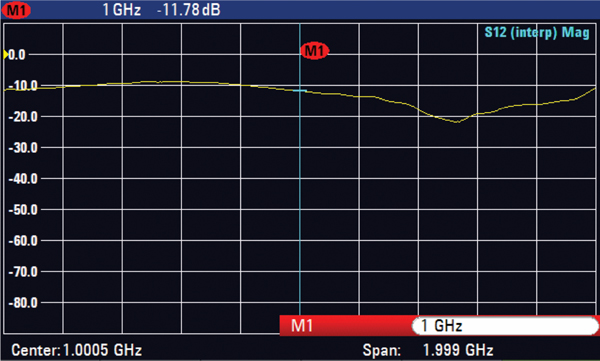
Screenshot Four: DC-9 Output Isolation with Poor Input Impedance
Screenshot Four measures isolation from the ‘tap’ to the ‘output’ port (same setup as in measurement three), with a poor impedance match on the input port. With a poor impedance match on the input port, isolation between the tap and output legs at 1GHz drops from 44.6 dB to 11.8 dB! This illustrates why the use of small value (distributed) pads is vital, as it helps to ensure that the proper impedance is seen at all ports and isolation values are kept at their best-case values.
As a final observation, many if not most modern spectrum analyzers that provide these measurements are only available with a 50 ohm characteristic impedance. This begs the question “How does one properly test with 50 ohm equipment in the HFC network where the characteristic impedance is 75 ohms”? The answer is “it’s not only possible, that’s how these measurements were taken;” but you’ll have to wait for Part II for further explanation as we examine frequency response and return loss measurements.
 H. Mark Bowers,
Cablesoft Engineering, Inc.
cablesofteng@gmail.com
Mark is VP of Engineering at Cablesoft Engineering, Inc. He has been involved in telephony since 1968 and the cable industry since 1973. His last industry position was VP of Corporate Engineering for Warner Cable Communications in Dublin, OH. Mark’s education includes the U.S. Naval Nuclear Engineering School, and BS and MS Degrees in Management of Technology. Mark is a member of the SCTE, the IEEE, and is a Senior Member and licensed Master Telecommunications Engineer with iNARTE.
Credit: Charts provided author
Credit: Shutterstock