Coaxial Cable Characteristics
By H. Mark Bowers
In my summer column we began a review of the research conducted by Oliver Heaviside (1850 to 1925), an English physicist, engineer, and mathematician whose research helped define our industry. If you’ve not read my last column covering resistance, reactance and impedance, you may wish to before proceeding. https://broadbandlibrary.com/resistance-reactance-and-impedance/
Coaxial cable basics
Most of us are familiar with coaxial cable, which has been deployed in cable television since the first systems were constructed in the 1940s and 1950s. Now let’s build on my last column with an examination of the coaxial transmission line. Coaxial cable has an inner conductor surrounded by a tubular insulating layer, surrounded by a tubular conducting shield. The term coaxial is used because the inner and outer conductors share a common geometric axis.
In 1880 Oliver Heaviside studied the so-called skin effect in telegraph transmission lines. He concluded that wrapping an insulating casing around a transmission line increased both the clarity of the signal and durability of the cable. He patented the first coaxial cable the following year (British Patent No. 1407). Four years later, in 1884, the first commercial coaxial cable was manufactured by Siemens. See Figure 1.
Coaxial cable is used to transport high frequency electrical signals with relatively low loss and is used in a variety of applications and industries. It differs from other shielded cables in that the dimensions of the cable conductors and connectors are more precisely controlled to provide for {the} efficient transfer of electrical energy from source to load while shielding the signal from outside interference.
In the analysis that follows, most coaxial cable parameters can be characterized by well established formulas; however, with the exception of characteristic impedance (Z0) we’ll not review them as mathematical analysis is not my general intent.
The outer sheath is usually maintained at ground potential, with the center conductor at some potential other than ground. As we might expect, coaxial cable operates in an intuitive fashion at lower frequencies (for example, 60 Hz) since it is simply two conductors separated by an insulating material. At higher frequencies, however, performance and analysis become complex.
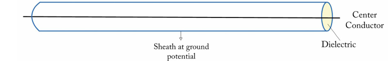
Figure 1. Coaxial cable construction
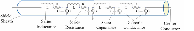
Figure 2. Equivalent coaxial cable at high frequency
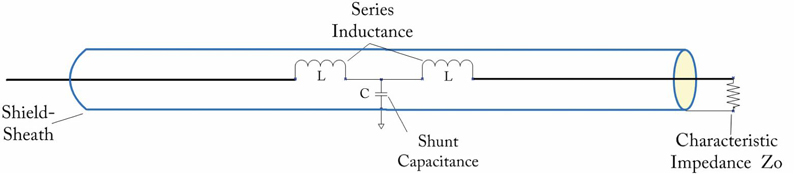
Figure 3. Simplified equivalent coaxial cable
Coaxial cable equivalent circuit
At higher frequencies, the coaxial cable takes on complex characteristics that can be best shown as a series of ‘distributed’ values of inductance, resistance, capacitance, and conductance. See Figure 2.
Coaxial cables are often analyzed as ‘lossy’ elements with lumped capacitance and inductance values, although the electrical performance of a length of coaxial cable transporting high frequency signals is more complex than this.
Series resistance
The DC resistance of a coaxial cable is provided per unit length, with the resistance of the center conductor and sheath usually given separately. For example, manufacturers published data for the resistance of .500” P3 cable is 1.35 ohms per 1k ft for the center conductor and .37 ohm per 1k ft for the sheath. Loop resistance is the sum of these values.
Series inductance
A length of coaxial cable, although straight, contains some inductance due to the magnetic field around the center conductor as energy is transferred. This magnetic field is represented as a series inductor specified in (micro) henries per unit length.
Shunt capacitance
Shunt capacitance represents the capability of the coaxial cable to carry a charge. Since the center conductor and sheath are separate conductors at different voltage potentials separated by a dielectric, a length of coax contains capacitance and is specified in (pico) farads per unit length.
Shunt conductance
Conductance is the opposite of resistance. It is the measure of how easily an electric current flows through a material. Conductance is designated by the letter G and is rated in siemens (S), or originally in mhos (Ʊ ohm spelled backwards) for us old timers. Mathematically, conductance is the reciprocal of resistance: G = 1/R. Generally, shunt conductance is small in coaxial cable because modern dielectric materials have excellent properties with a low dielectric constant. At higher frequencies, however, the dielectric will allow some conductance (leakage) between the center conductor and the sheath.
Dielectric loss
Dielectric losses arise from energy absorption as the electric field rapidly changes polarity and occurs when conductance is greater than zero. It represents one of the major losses in coaxial cable at high frequencies. The energy lost is dissipated as heat, and increases directly with the applied frequency (and applied RF voltage).
RF attenuation
At higher frequencies skin effect increases the effective AC resistance by confining conduction to a thin outer layer of each conductor. In addition to the increase in resistive loss, where high frequencies exist the effect of dielectric loss becomes significant as well. I’m not including a formula for calculation of RF attenuation, because in my experience the calculated results often vary significantly from the manufacturer’s published data for a variety of reasons. So, always use the manufacturer’s published RF attenuation data when available.
Characteristic impedance
As discussed in my last column, impedance represents the total opposition to current flow and includes the effects of resistance along with inductive and capacitive reactance. Because reactive components are often present (unless the circuit is resistive only), impedance is usually a complex value, meaning it has both magnitude and phase components. Most manufactured cables (including non-coaxial) have a specified characteristic impedance Z0. The Z0 of a transmission line of infinite length is the impedance in ohms at a specified frequency.
Characteristic impedance has valuable application that can be more readily understood in terms of its effect on source-to-load energy transfer. If the input of a coaxial cable with a Z0 of 75 ohms is connected to a signal source with 75 ohm impedance and the output of the cable is connected to a 75 ohm resistive load, all energy is transferred from source to load (zero reflected energy). We will examine this idea further in my next column.
In coaxial cable Z0 is determined by the cables’ resistance, capacitance, inductance and conductance as shown in the following formula.
![]() where:
where:
Z0 = characteristic impedance (ohms)
R = series resistance per unit length (ohms)
L = series inductance per unit length (henrys)
G = conductance per unit length (siemens)
C = shunt capacitance per unit length (farads)
j = angular momentum (phase) introduced by the inductive and capacitive components
Now examine Figure 3. Since the resistive (R) and conductive (G) components in modern coaxial cable are relatively low compared to other factors, the first Z0 formula can be simplified to
![]()
for a lossless line. Note that the ratio of L/C must remain approximately 5625 to yield a Z0 of 75 ohms for cable television application. This ratio between series inductance and shunt capacitance arises from the ratio of the spacing between the inner and outer conductors plus the type and quality of dielectric material. This yields a third formula which will be familiar to many of you.
![]()
where:
εk = dielectric constant
D = inside diameter of the outer conductor (sheath) in inches or mm.
d = outside diameter of the inner conductor (center conductor) in inches or mm.
Using .500” P3 cable as an example, a εk of 1.3 (modern foam dielectric) plus .452” for D and .109” for d yields a Z0 of 74.76 ohms.
In my winter 2020 column we’ll use the concepts from my spring and summer columns to make some further observations on coaxial transmission lines including several measurements.
 H. Mark Bowers,
Cablesoft Engineering, Inc.
Mark is VP of Engineering at Cablesoft Engineering, Inc. He has been involved in telephony since 1968 and the cable industry since 1973. His last industry position was VP of Corporate Engineering for Warner Cable Communications in Dublin, OH. Mark’s education includes the U.S. Naval Nuclear Engineering School, and BS and MS Degrees in Management of Technology. Mark is a member of SCTE•ISBE, IEEE, and is a Senior Member and licensed Master Telecommunications Engineer with iNARTE.