Coaxial Cable Testing
By H. Mark Bowers
In my summer and fall columns we reviewed the following transmission line characteristics: resistance, reactance, impedance, series resistance and conductance, shunt capacitance and conductance, dielectric loss, RF attenuation, and characteristic impedance. Before we can review testing procedures for coaxial cable there are several remaining parameters to touch on: velocity factor, wave motion, reflections and standing waves. These reviews must be kept to an overview due to space restrictions. An unabridged version of this report will be available on my website and will address these issues in greater depth, especially standing waves. See www.cablesoftengineering.com/downloads/.
Velocity factor
Velocity factor (VF) is the speed at which an electrical signal propagates through a cable relative to the speed of light, expressed in decimal form. In a vacuum the VF is 1. If VF is .7 the signal in the cable propagates at 0.7 times the speed of light. When VF is expressed as a percentage, it’s called velocity of propagation. VF is calculated by the formula
![]()
where ϵ is the dielectric constant of the dielectric material. VF in a coaxial cable is therefore determined by the dielectric material in use. There are a number of materials that have been used for dielectric over the years. Each has a different dielectric constant and thus yields a different VF. Common values for dielectric constant are 2.3 for solid polyethylene (PE) yielding a VF of 0.66, and the more recent 1.3 for modern foam polyethylene yielding a VF of 0.87.
Wave motion on an infinite line
Figure 1 illustrates voltage (E) and current (I) sine waves that travel at speed VF along a transmission line of infinite length.
Because the line is of infinite length no reflections occur, therefore, the voltage and current remain in-phase along the entire line. Due to line losses, the wave peaks diminish in amplitude as the waves propagate along the line length. Figure 1 illustrates what would happen if E and I were stopped for a moment in time. In this figure the waves are stopped at the instant when the AC source voltage reaches zero. An instant later the waves would shift slightly to the right.
Traveling waves exist on the transmission line because it takes a finite amount of time for them to propagate down the line. The characteristics of a theoretically infinite line are informative and can be summarized as:
- E and I are in-phase along the entire line length.
- The ratio of the amplitude of E to I is constant along the entire length and is the characteristic impedance (Z0).
- The input (source) impedance is equal to the line characteristic impedance (Z0).
- Since E and I are in-phase, the line operates at maximum efficiency.
- Any line length can be made to appear infinite if it is terminated in its characteristic impedance.
Line reflections
A signal travelling down a transmission line will be partly (or wholly) reflected back in the opposite direction when the travelling signal encounters a discontinuity in the characteristic impedance, or if the far (load) end of the line is not terminated properly. Reflections cause undesirable effects including inefficient transfer of signal power and modified frequency response. Reflections create standing waves on the line. Conversely, standing waves are an indication that reflections are present.
Return loss is one way to characterize impedance mismatches, and is the ratio in decibels of power incident upon an impedance discontinuity to the power reflected by the discontinuity. Mathematically, where RL is the return loss in dB, PI is the incident power and PR is the reflected power. A higher RL indicates an improved impedance match (lower magnitude reflections), which results in lower insertion loss. Return loss is a positive number as long as PI > PR.
![]()
Common coaxial testing methods
Common coaxial testing methods include use of a time domain reflectometer (TDR), RF loss measurements at specific or multiple frequencies, DC resistance, summation sweeping, adaptive equalizer activity (in digital signals), return loss and standing waves. We will briefly examine the last two.
Actual measurements
For my measurements I employed a medium quality spectrum analyzer (50 ohm input impedance) with internal tracking generator along with an external return loss bridge (RLB) of fair quality. If you wish to learn more about how to perform these tests you’ll need to search for articles on this subject.
Measurements were performed on a length of Series 6 coaxial cable with an undetermined discontinuity towards the end of the run. I built a new home in the fall of 2019 and one Series 6 run is partially shorted in a finished basement ceiling. I tried a TDR and a high quality leakage detector in an attempt to pinpoint the damage with less than satisfactory results. In Figure 4 we’ll use standing waves as a third method.
Return loss measurements
See Figure 2. I have the tracking generator and spectrum analyzer connected to the return loss bridge using high quality jumpers. I normalized the trace to the top graticule line to account for jumper and connector loss, matching pad loss, and any small discontinuities at the source. I then placed a 75 ohm terminator at the DUT (device under test) port on the RLB to establish a baseline for these tests. Dynamic range is limited due to the matching pad loss plus the lack of a high quality RLB. It is, however, adequate for these tests. The best case RL was approximately 29 dB. Note: These numbers appear negative in the marker table because each value is referenced to the top (normalized) graticule; however, as already noted RL is a positive value.
Now examine Figure 3. I noted earlier that a higher return loss is desirable as it indicates less reflected power. The higher return loss measured with the 75 ohm terminator has now dropped to 4 dB to 16 dB depending on frequency. There is clearly a great deal of reflected energy present on this line as expected.
Standing wave measurements
Standing waves are created by the addition and subtraction of the incident and reflected waves at a given point on the transmission line. In Figure 4 we see the results of feeding the tracking generator signal into the defective cable using a directional coupler to measure the combined forward and reflected signals. Positive peaks every 5.2 MHz can be seen on the waveform. The relationship between the frequency between successive peaks, velocity factor, and distance to the fault is shown by the formula:
![]()
where DTF is distance to fault in feet, VF is the velocity factor, and VP is the distance between standing wave peaks in MHz. Using 5.2 MHz for DP and 0.87 for VF yields a DTF of 83.32 ft.
Final thoughts
In these past three articles I’ve reviewed many of the parameters associated with signal transport on transmission lines in general and coaxial cable more specifically. Operation at higher frequencies is far more complex than one might expect. As a concluding anecdote, using this standing wave method to estimate DTF can be quite accurate if measured at lower frequencies, especially in the return path. Using this method some years back during a return path proof-of-performance led me to within 6 ft of a defective splice. The local plant technician was duly impressed.
—
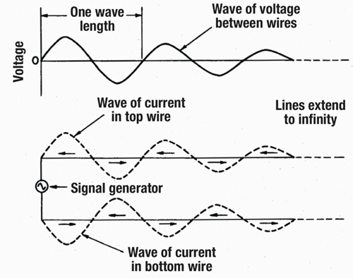
Figure 1. Traveling waves of current and voltage
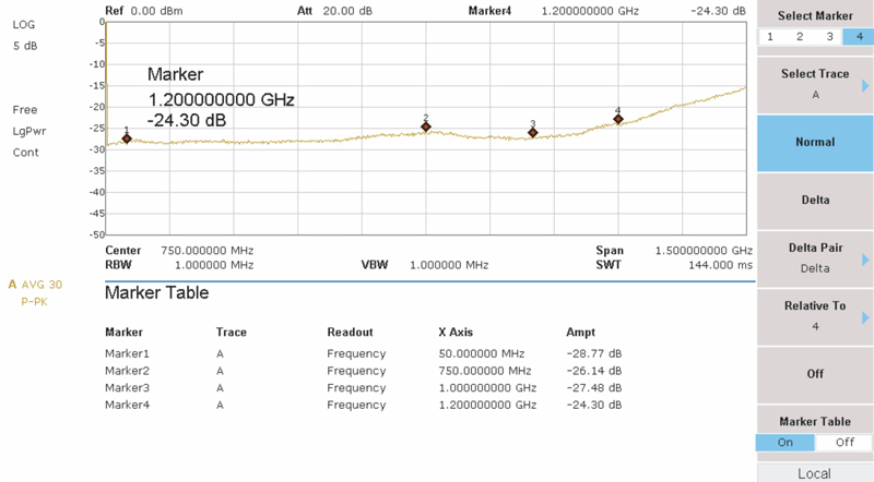
Figure 2. Return loss with a termination on the DUT port
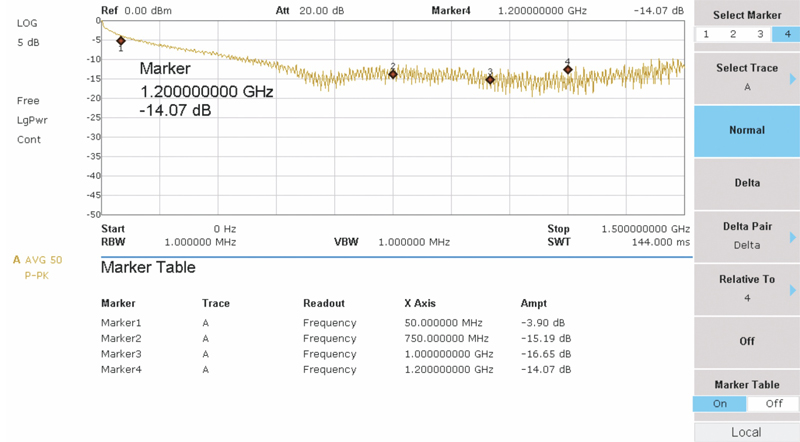
Figure 3. Return loss on defective Series 6 cable
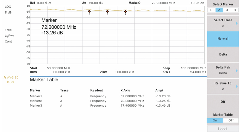
Figure 4. Standing waves on defective Series 6 cable run
 H. Mark Bowers,
Cablesoft Engineering, Inc.
Mark is VP of Engineering at Cablesoft Engineering, Inc. He has been involved in telephony since 1968 and the cable industry since 1973. His last industry position was VP of Corporate Engineering for Warner Cable Communications in Dublin, OH. Mark’s education includes the U.S. Naval Nuclear Engineering School, and BS and MS Degrees in Management of Technology. Mark is a member of SCTE•ISBE, IEEE, and is a Senior Member and licensed Master Telecommunications Engineer with iNARTE.