Signal Leakage Field Strength
By Ron Hranac
Cable operators for decades have dealt with the monitoring and measurement of signal leakage field strength. But just what is field strength?
The measurement of signal leakage is fairly straightforward: Using a dedicated leakage detector (typically with a built-in antenna), orient the detector and its antenna to get a maximum reading and see what value the leakage detector reports. The measured field strength is stated in microvolts per meter (µV/m) [1], and hopefully is below the maximum limit defined by government regulations for the frequency range of interest. Table 1, from §76.605(c) of the FCC Rules, summarizes leakage limits and measurement distances applicable to U.S. cable networks.
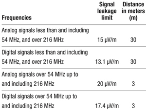
Table 1. FCC signal leakage limits
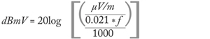
Sometimes leakage is measured using a resonant half-wave dipole antenna connected to a signal level meter or spectrum analyzer (often with a bandpass filter and preamplifier in between; more on this later). When using this technique, the instrument’s reported value in dBmV must be converted to field strength in µV/m. First, compensate for the insertion loss of the interconnecting cable(s) and external bandpass filter, as well as the gain of the preamplifer, to determine the signal level in dBmV at the antenna’s terminals. Then use the following formula to convert to µV/m.
µV/m = 20 * f * 10(dBmV/20)
where
µV/m is field strength in microvolts per meter
f is the leakage measurement frequency in MHz
dBmV is the signal level at the dipole’s terminals.
Conversely, one can use the following formula to convert a known field strength in µV/m to dBmV at the dipole’s terminals:
But that still doesn’t explain what field strength is. Things get even more confusing when measuring leakage on more than one frequency. Assuming the same field strength — say, 20 µV/m — at two frequencies and the use of separate resonant half-wave dipoles for the measurements, the dBmV values at the two dipoles’ terminals will be different. For example, a field strength of 20 µV/m at 121.2625 MHz will produce -42.1 dBmV at the terminals of a resonant half-wave dipole for that frequency. A field strength of 20 µV/m at 782 MHz will produce -58.29 dBmV at the terminals of a resonant half-wave dipole for that frequency.
To understand what’s happening, consider the following example, based upon the assumptions in Table 2.
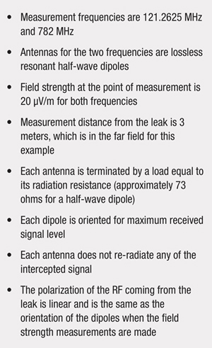
Table 2. Assumptions for example
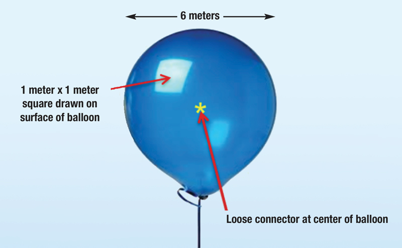
Figure 1. Loose connector inside of 6 meter diameter balloon, radiating RF outwards equally in all directions and “illuminating” the balloon from the inside.
Visualize a loose connector radiating RF into the space around it. Now imagine a 6-meter diameter balloon surrounding the loose connector, with the loose connector at the center of the balloon. Assume the RF leaking from the loose connector is uniformly “illuminating” the entire surface of the balloon from the inside (see Figure 1). Next, imagine a 1 meter x 1 meter square drawn somewhere on the surface of the balloon.
The task at hand is to measure the RF power density within the 1 meter x 1 meter square. The power density in that square also can be expressed as a voltage, which is how field strength is expressed: volts per meter. In other words, field strength is the RF power density in a 1 meter x 1 meter square (in free space, in the air, or, as in this example, on the surface of an imaginary 6-meter diameter balloon), expressed as a voltage — hence, the “volts per meter” or “microvolts per meter” designation.
Let’s do some number crunching to help clarify things. The RF power “transmitted” by the loose connector in the center of the balloon is designated Pt, and is called the source power. In order to produce a field strength of 20 µV/m 3 meters away, Pt must equal 0.00000000012 watt or 1.2 * 10-10 watt (in case you’re wondering, I calculated Pt in advance for this example by working backwards from 20 µV/m). Because the RF source power Pt is uniformly illuminating the entire balloon (an analogy is a light bulb at the center of the balloon), the power density Pd on the surface of the balloon in watts per square meter is simply the source power Pt divided by the surface area of the balloon, or
Pt /4πr2
where r is the radius of the balloon. Since the balloon’s diameter is 6 meters, r = 3 meters. Plugging the just-discussed values for Pt and r into the formula, the calculated power density on the surface of the balloon is equal to about 1.06 * 10-12 watt per square meter (the actual value is 0.00000000000106103295 watt per square meter).
The impedance Z of free space is 120π ohms [2], or about 377 Ω. Using the formula
![]()
the voltage V on the surface of the balloon in volts per meter is
![]()
= 0.000020 volt per meter, or 20 µV/m.
So far, so good: A source power Pt of 1.20 * 10-10 watt transmitted by the loose connector illuminates the surface of the balloon 3 meters away to produce a power density Pd of about 1.06 * 10-12 watt per square meter, which is equal to a field strength of 20 µV/m. This relationship is true for both frequencies (121.2625 MHz and 782 MHz).
Next, the resonant half-wave dipoles for the two frequencies are placed one at a time in the square on the surface of the balloon, and the field strength within that square measured. The question is how much of the RF power in the square is intercepted by each dipole and delivered to the load connected to each antenna’s terminals? All of it? Only an amount occupying an area equal to the physical dimensions of each antenna? Or some other amount?
Visualize what happens when a dipole is placed at the surface of the balloon, where RF from the loose connector 3 meters away is passing by at the speed of light. The RF field induces a voltage V in the dipole, resulting in a current I through the approximately 73 Ω impedance connected to the antenna terminals. What’s of interest is the power P delivered by the antenna to that impedance, where P = I2RT. Here RT is the sum of the antenna’s radiation resistance (~73 ohms) and loss resistance, the latter assumed to be zero for this example. The book Antennas, Second Edition [3] illustrates a scenario using a horn antenna.
Let the…power density of the plane wave be S watts per square meter and the area of the mouth of the horn be A square meters. If the horn extracts all the power from the wave over its entire area A, then the total power P absorbed from the wave is P = SA (W). Thus, the electromagnetic horn may be regarded as an aperture…
The same is true of a dipole antenna — that is, it can be regarded as an “aperture” with a specific area that extracts power from a passing wave and delivers it to the load connected to the antenna’s terminals. Defining aperture isn’t quite as simple as one might assume, though. According to Antennas, Second Edition, three types of aperture describe
…ways in which power collected by the antenna may be divided: into power in the terminal resistance (effective aperture); into heat in the antenna (loss aperture); or into reradiated power (scattering aperture).
A fourth aperture, called collecting aperture, is the sum of the three previous apertures. Finally, physical aperture is basically “a measure of the physical size of the antenna,” but surprisingly doesn’t have all that much to do with how much power is actually intercepted by an antenna.
Since the dipoles in this example are assumed to be lossless, effective aperture — more specifically, maximum effective aperture Aem — is the criteria that will be used to describe how much of the RF power in the 1 meter x 1 meter square is intercepted and delivered to the load at the antenna terminals. Mathematically
Aem = (λ2 ⁄ 4π)G
where λ is wavelength in meters (299.792458/fMHz) and G is the antenna’s numerical gain (1.64 for a half-wave dipole). A linear half-wave dipole’s maximum effective aperture is an elliptically shaped aperture with an area equal to 0.13λ2, as shown in Figure 2.
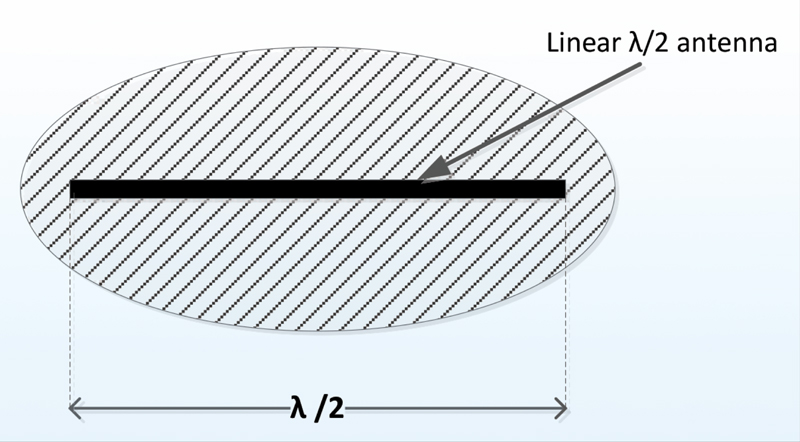
Figure 2: A linear half-wave dipole’s maximum effective aperture Aem is represented by an ellipse with an area of 0.13λ2. (After Kraus, J., Antennas, 2nd Ed.)
The free-space wavelength for 121.2625 MHz is approximately 2.47 meters (2.47226024534) and for 782 MHz is approximately 0.38 meter (0.383366314578). Plugging these numbers into the previous formula gives a maximum effective aperture of 0.797668339532 m2 for the 121.2625 MHz dipole, and 0.0191805865422 m2 for the 782 MHz dipole. The Aem values denote what percentage of the power within the 1 meter x 1 meter square is intercepted by each dipole and delivered to the load at the antenna terminals. Recall that the power density Pd on the surface of the balloon is ~1.06 * 10-12 watt per square meter. The power intercepted by the two antennas and delivered to the ~73 Ω load at their terminals is ~79.8% of Pd for the 121.2625 MHz dipole and ~1.9% of Pd for the 782 MHz dipole, or ~8.46 * 10-13 watt and ~2.04 * 10-14 watt respectively.
Going back to the maximum effective aperture of the two antennas, the difference between the two Aem values in decibels is
10log(Aemdipole 1 /Aemdipole 2)
or 16.19 dB, which is equal to the antenna factor [4] difference between the two dipoles.
In other words, when measuring a 20 µV/m field strength at 121.2625 MHz and 782 MHz with resonant half-wave dipoles, the lower frequency antenna intercepts and delivers more power to its load (~8.46 * 10-13 watt) than the higher frequency antenna does (~2.04 * 10-14 watt). Here, too, the decibel difference is the same as the antenna factor difference. All of this jibes with the two different signal levels at the dipoles’ terminals: -42.1 dBmV at 121.2625 MHz and -58.29 dBmV at 782 MHz, for the same 20 µV/m field strength at the two frequencies.
The different antenna factors for the 121.2625 MHz and 782 MHz dipoles equate to an effective loss of RF sensitivity in the UHF range compared to the VHF range, by an amount equal to the antenna factor difference (16.19 dB in the previous example). This is why a half-wave dipole and spectrum analyzer combination by itself for UHF leakage detection is usually inadequate, especially when attempting to measure low-level leakage. More often than not, one will need a higher gain antenna than a dipole and possibly also a bandpass filter and preamplifier to improve overall equipment sensitivity (the same may be true at lower frequencies, depending on the leakage field strength). Otherwise the low- to moderate-field strength signal leakage may be hidden beneath the test equipment’s noise floor.
So, what does all of this tell us about field strength? It’s the RF power density in a 1 meter x 1 meter square — as mentioned previously, in free space, in the air, on the surface of an imaginary balloon — expressed as a voltage (more specifically, our familiar microvolts per meter).
This article was adapted from “UHF Signal Leakage and Ingress: Understanding the Challenges,” a Technical Workshop Paper by Ron Hranac and Nick Segura; SCTE Cable-Tec Expo ’13, October 21-24, 2013, Atlanta, GA
Notes:
[1]Outside of the North American cable industry, field strength measurements are more commonly stated in decibel microvolts per meter, or dBµV/m
[2]https://en.wikipedia.org/wiki/Impedance_of_free_space
[3]Antennas, Second Edition, by John D. Kraus (© 1988, McGraw-Hill, Inc., ISBN 0-07-035422-7)
[4]The antenna factors for the VHF and UHF dipoles in this example are 8.12 dB/m and 24.31 dB/m respectively. For more information about antenna factor, see “The Antenna Factor,” published in the 3Q12 issue of Communications Technology, available on-line HERE.
 Ron Hranac
Technical Marketing Engineer,
Cisco Systems
rhranacj@cisco.com
Ron Hranac, a 46-year veteran of the cable industry, is TME for Cisco’s Cable Access Business Unit. A Fellow Member of SCTE, Ron was inducted into the Society’s Hall of Fame in 2010, is a co-recipient of the Chairman’s Award, an SCTE Member of the Year, and is a member of the Cable TV Pioneers Class of ’97. He received the Society’s Excellence in Standards award at Cable-Tec Expo 2016. He has published hundreds of articles and papers, and has been a speaker at numerous international, national, regional, and local conferences and seminars.