Radio Frequency
By Ron Hranac
The cable industry has used RF in its networks for decades, but if someone were to ask you to explain RF, how would you answer? Numerous books, papers, and articles have been written on the subject, and countless classes taught in schools around the world. The engineering side of RF can get rather gnarly, so let’s start with the easy part: Spelling out the abbreviation gives us radio frequency, but now we have to figure that out! I have three definitions:
- “Radio frequency” is that portion of the electromagnetic spectrum (see Figure 1) from a few kilohertz to just below the frequency of infrared light (~3 kHz to ~300 GHz). Note: Some radio communications with submarines has been done on frequencies as low as about 80 Hz. Radio communications at 300 GHz is limited to maybe a few meters, because the atmosphere is essentially opaque to radio signals at that frequency. The coaxial cable portion of our networks uses frequencies from 5 MHz to 1218 MHz (1.2 GHz) or higher.
- “Radio frequency” can describe the type of signal that occupies the aforementioned portion of the electromagnetic spectrum. For instance, the hardline coaxial cable in our networks carries single carrier quadrature amplitude modulation (SC-QAM) RF signals along with 60 or 90 volts AC, the latter to operate the nodes and amplifiers (by the way, the RF current inside of coaxial cable also is alternating current, just a lot higher in frequency).
- “Radio frequency” can be defined as a rate of oscillation within the 3 kHz to 300 GHz range. I’ll get back to that in a moment.
NASA defines the electromagnetic spectrum as “…the range of all types of electromagnetic radiation.” (For more about the electromagnetic spectrum, see https://imagine.gsfc.nasa.gov/science/toolbox/emspectrum1.html#:~:text=The%20Electromagnetic%20Spectrum,two%20types%20of%20electromagnetic%20radiation)
Electromagnetic radiation is a form of energy comprising oscillating electric and magnetic fields. The electric and magnetic components are orthogonal (perpendicular) to each other, and also are orthogonal to the direction of propagation. Electromagnetic radiation can be visualized as waves, analogous to the ripples that occur when one tosses a rock into a pond of water. Here are some more definitions related to the electromagnetic spectrum. Figure 2 illustrates the first three definitions
- Frequency — The number of times, typically per second, that a repetitive event happens; that is, the previously mentioned rate of oscillation of an electromagnetic signal. Frequency is measured or stated in units of hertz (Hz), which is the number of cycles or waves per second; see Table 1. Back to the pond analogy: Throw a rock in the water, then count the number of waves per second that go by a wooden post sticking out of the water. That’s the frequency.
- Amplitude — The intensity or strength of an electromagnetic signal (more on this later). An analogy is the height of those ripples on the water.
- Bandwidth — The amount (width) of spectrum, measured in units of Hz, that an electromagnetic signal occupies. (The data side of the world co-opted “bandwidth” to mean data rate or data capacity, but being an RF guy I prefer the definition here.)
- Wavelength — An electromagnetic signal’s speed of propagation divided by its frequency in cycles per second. If you could see the electromagnetic signal’s waves, wavelength would be the distance from a point on one cycle’s wave to the same point on the next cycle’s wave. Going back to the pond analogy, measure the distance between adjacent ripples’ peaks or valleys to determine the wavelength. Mathematically, an electromagnetic signal’s wavelength is related to its frequency by the formula
Wavelength (λ) in meters = 299.792458 ÷ frequency in MHz
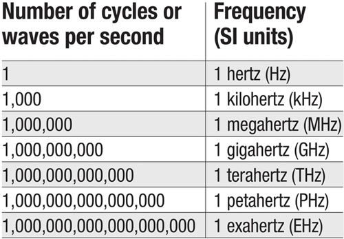
Table 1. Cycles per second and frequency
Unlike the visible light portion of the electromagnetic spectrum, RF can’t be seen. Its presence and various characteristics such as frequency, wavelength, and amplitude can be detected and measured with specialized test equipment such as signal level meters and spectrum analyzers.
RF energy propagates through a vacuum at the speed of light (186,282.4 miles per second) and is made of photons. The same is true of gamma rays, X-rays, and light, all of which are forms of electromagnetic radiation.
An RF signal can convey information using modulation to vary one or more characteristics of that signal: its amplitude, frequency, and/or phase.
Getting RF from here to there
RF signals can be transmitted from one point to another using a variety of media: over-the-air; twinlead (remember connecting a rooftop antenna to a TV with twinlead?); window line and ladder line (similar to twinlead); microstrip (used on printed circuit boards); and waveguide (used at microwave frequencies). The cable industry, of course, uses coaxial cable.
RF signal level
Signal level is the amplitude of a signal, specifically its power. An important point: Signal level in cable networks is expressed in dBmV (not dB). Want to learn more? See https://broadbandlibrary.com/wise-and-mighty-decibel/.
Coaxial cable attenuation-versus-frequency
Some interesting things happen to RF as it travels through coaxial cable. One phenomenon is higher attenuation at higher frequencies. Because of something known as skin effect, RF travels on and near the surface of the center conductor and inside of the shield. At higher frequencies the skin depth decreases, making the effective cross section of the conductor less! That means the RF “resistance” (and the cable’s attenuation) increases at higher frequencies, too. For more about this, see https://broadbandlibrary.com/skin-effect-and-skin-depth/.
Velocity of propagation
What we call velocity of propagation in coax is the percentage of the free space value of the speed of light that the RF is traveling. So, coax with a VP of 87% means that the RF is traveling 162,065.69 miles per second in the cable (1 foot in 1.17 nanosecond), compared to the free space value of 186,282.4 miles per second. Several years ago I wrote an article with a deep dive explanation, available on SCTE·ISBE’s web site at https://scte-cms-resource-storage.s3.amazonaws.com/10-03-01%20velocity%20of%20propagation.pdf
Coaxial cable attenuation-versus-temperature
Coax attenuation in decibels varies about 1 percent per 10 °F of temperature change; so over temperature, RF signal levels in coax also change. The reason? Hint: It’s not because of the expansion and contraction of the cable. Instead, it has to do with processes in the metallic conductors occurring at the atomic level. I wrote an article about this in the April 2002 issue of Communications Technology magazine. Unfortunately, that article is not available on-line as far as I know, so you’ll have to dig through your collection of back issues.
There is a whole lot more to the topic of RF than I can possibly cover here, and I’ve barely scratched the surface. RF has been an important part of cable networks since the very first CATV systems were built in 1948. The “C” (coax) part of our HFC networks uses RF to distribute and transport signals. Wi-Fi and other wireless technology — which use RF — are part of cable’s service offering, too! RF will be part of the cable industry’s networks for the foreseeable future, helping us deliver video, voice, and multi-gigabit data services.
—
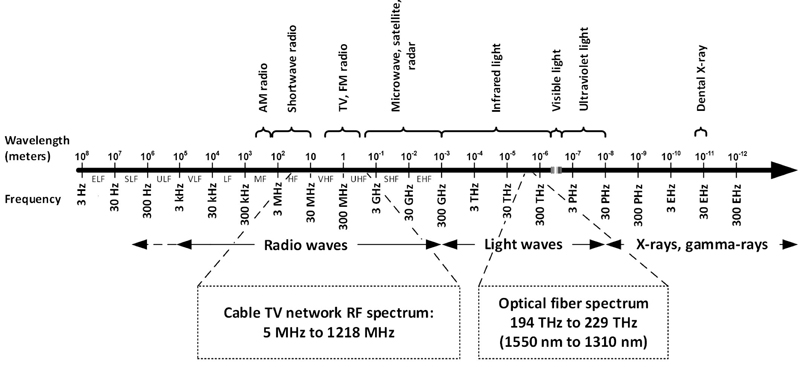
Figure 1. The electromagnetic spectrum. What we call RF encompasses “radio waves,” which extend from about 3 kHz to 300 GHz (see text).
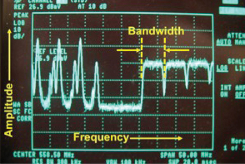
Figure 2. Spectrum analyzer display showing analog TV signals (left side) and SC-QAM signals (right side). The horizontal axis is frequency and the vertical axis is amplitude. The amount of spectrum occupied by a signal is its bandwidth, expressed in Hz, kHz, MHz, etc. Here, each analog TV signal and SC-QAM signal has a bandwidth of 6 MHz — that is, each one is 6 MHz wide.
 Ron Hranac
Technical Marketing Engineer,
Cisco Systems
rhranacj@cisco.com
Ron Hranac, a 47 year veteran of the cable industry, is Technical Marketing Engineer for Cisco’s Cable Access Business Unit. A Fellow Member of SCTE and co-founder and Associate Board Member of the organization’s Rocky Mountain Chapter, Ron was inducted into the Society’s Hall of Fame in 2010, is a co-recipient of the Chairman’s Award, an SCTE Member of the Year, and is a member of the Cable TV Pioneers Class of ’97. He received the Society’s Excellence in Standards award at Cable-Tec Expo 2016. He was recipient of the European Society for Broadband Professionals’ 2016 Tom Hall award for Outstanding Services to Broadband Engineering, and was named winner of the 2017 David Hall Award for Best Presentation. He has published hundreds of articles and papers, and has been a speaker at numerous international, national, regional, and local conferences and seminars.