Signal Level: The Powers That Be

Current is the flow of charged particles through a conductor, measured as the net rate of flow of those charged particles (i.e., flow per unit of time). Ampere, abbreviated A, is a measure of electric current; 1 ampere equals 1 coulomb of charge flowing past a given point in 1 second. [Note: Coulomb is the International System of Units (SI) derived unit of electric charge, where 1 coulomb is defined as 10¹⁹/1.602176634 elementary charges. An “elementary charge” is the magnitude of the charge of an electron, but the electron charge is negative; as such, the charge of one electron is approximately 1.602 * 10^-19 coulombs.] An analogy for current is the volume of water flowing through a garden hose, such as 1 gallon of water per second.

Voltage is the difference in electric potential between two points. The volt, abbreviated E or V, is a derived unit for electric potential (or electromotive force, EMF), where 1 volt is the potential difference between two points on a conductor (wire) carrying 1 ampere of current when the power dissipated between the points is 1 watt. Voltage is analogous to water pressure in a garden hose, such as 1 pound per square inch (PSI). [Note: EMF is the force of electrical attraction between two points of different charge potential.]

Resistance (R) is an opposition to the flow of current. Ohm, abbreviated Ω, is a unit of resistance, where 1 ohm is defined as the resistance that allows 1 ampere of current to flow between two points that have a potential difference of 1 volt. A garden hose analogy is squeezing or kinking the hose to oppose the flow of water.

Ohm’s Law

The definition for resistance is part of the basis for Ohm’s Law, which is R = E/I. Here R is resistance in ohms, E is electromotive force in volts, and I is current in amperes. (Current is abbreviated I for intensité de courant. Why not C? That letter is used as an abbreviation for capacitance and coulomb.) The formula R = E/I can be shuffled around a bit to give us some of the other variations of Ohm’s Law: E = IR and I = E/R. Figure 1 shows an easy way to remember the three Ohm’s Law formulas.

Using Ohm’s Law, we can look at an example with 0.010 volt or 10 millivolts (mV) across a 75 ohms resistance (see Figure 2), and calculate the current:

I = E/R

I = 0.010 volt/75 ohms

I = 0.000133 ampere, or 0.133 milliampere (mA)

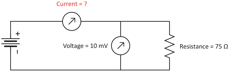
Figure 2. Calculating current in a DC circuit

Power

Power is the rate at which work is done, or energy per unit of time, where 1 watt of power is equal to 1 volt causing a current of 1 ampere. Watt is the power required to do work at a rate of 1 joule per second (J/s). That is, a joule of work per second is 1 watt. 1 joule is the work done by a force of 1 newton acting over a distance of 1 meter. The joule is a measure of a quantity of energy and equals 1 watt-second.

The electric utility meter on the side of your house measures units of kilowatt-hour (kWh), which equals the amount of energy “used” by a load of 1 kilowatt (1,000 watts) over a period of 1 hour, or 3.6 million joules.

In other words, 1 watt is simply the use or generation of 1 joule of energy per second. Other electric units are in fact derived from the watt. For instance, 1 volt is 1 watt per ampere. Another definition of 1 watt is 1 volt of potential “pushing” 1 ampere of current through a resistance, or P = EI. As was the case with Ohm’s Law, a bit of formula shuffling will give us E = P/I and I = P/E.

Using your scientific calculator and some basic algebra, substituting the Ohm’s Law equivalents for E and I into the formula P = EI gives two other common expressions of power: P = E²/R and P = I²R.

Power in DC circuits

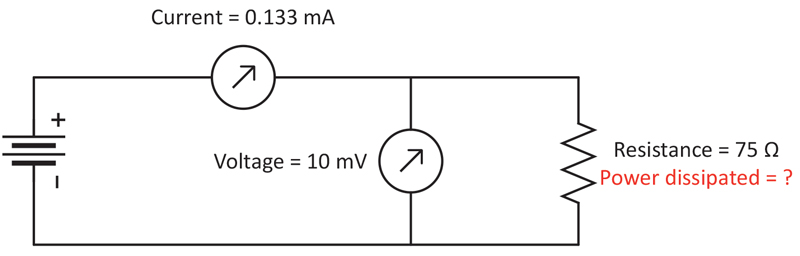
Power calculations and measurements in direct current (DC) circuits and applications are relatively straightforward. For example, if you have a 75 ohms resistor with an applied voltage of 10 millivolts, the power dissipated by the resistor is 1.33 microwatt (P = E²/R = 0.010²/75 = 1.33 * 10^-6 watt or 1.33 µW), as shown in Figure 3.

Power in AC circuits

Because the previous example is a DC circuit, the voltage always will be 10 millivolts and the current 0.133 milliampere. As long as the resistor’s value remains constant, it’s easy to calculate dissipated power. Alternating current (AC) circuits — including RF circuits — and applications are more complicated because the instantaneous voltage and current are not constant. In order to equate a varying AC waveform to a DC equivalent component, one must work in the world of root mean square (RMS) voltage and current.

In an AC circuit, the instantaneous values of voltage and current are varying continuously over time. How can we define useful values for these varying quantities? Root mean square gives us effective quantities equivalent to DC values. That is, RMS equates the values of AC and DC power to heat in a resistor by the same amount. [Note: RMS value is found by squaring the individual values of all the instantaneous values of voltage or current in a single AC cycle. Calculate the average of those squares and then calculate the square root of the average.]

For instance, 10 mV RMS AC voltage causes the same average power dissipation in a given resistor as does a 10 mV DC voltage. Likewise, 0.133 mA RMS alternating current has the same heating effect as 0.133 mA direct current. Root mean square values simplify calculations by making the product of RMS voltage and RMS current equal to average power:

Pavg = Erms * Irms * cos θ

where cos θ is the cosine of the phase angle between the current and voltage, also known as power factor. In a purely resistive circuit where voltage and current are in phase, the formula is Pavg = Erms * Irms.

Consider measurement of the power of an unmodulated sinusoidal RF carrier — commonly called a continuous wave or CW carrier — which is an AC waveform. AC power measurement can be a bit tricky, because the product of voltage and current varies during the AC cycle by twice the frequency of the sine wave.

In other words, the output of a signal source such as a sinusoidal RF signal generator is a sine wave current at the desired frequency, but the product of the signal’s voltage and current has what amounts to an equivalent average DC component along with a component at twice the original frequency. In most cases of RF power measurement, “power” refers to the equivalent average DC component of the voltage and current product.

If you connect a thermocouple power meter to the output of an RF signal source, the power meter’s power sensor will respond to the RF carrier’s DC component by averaging. The averaging usually is done over many cycles, which, at RF, still can be a relatively short period of time. Otherwise, if the power meter simply measured an instantaneous point of the sine wave, then measured that sine wave at another instantaneous point, the reported power value would vary according to the instantaneous product of the voltage and current at each measurement point. This is the primary reason why many RF carrier power measurements are expressed in average power.

Signal level

Imagine a sine wave viewed in the time domain — that is, amplitude versus time, as might be seen on an oscilloscope. See Figure 4.

 

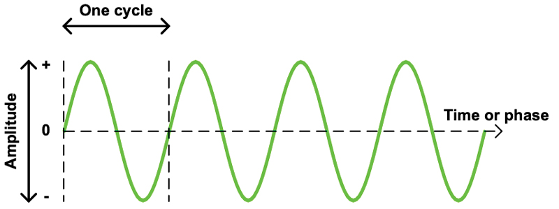
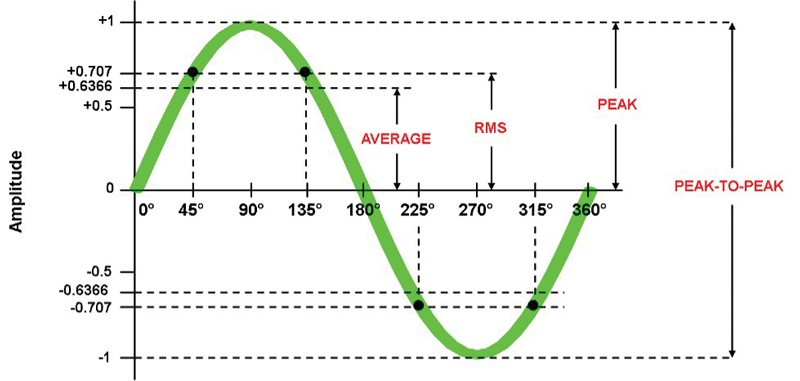
The AC waveform’s amplitude or level can be characterized in a variety of ways. For instance, we can measure the sine wave’s peak-to-peak, peak, RMS or average values of current and voltage, as illustrated in Figure 5 for a sine wave with a normalized peak value of 1. [Note: The actual average, mathematically speaking, of one cycle of a sine wave is zero. However, often in electrical discussions and literature there is mention of “average” for a sine wave, and those discussions have in mind the average value of a full-wave-rectified sine wave over one complete cycle. For a sine wave with peak value p, this average of the rectified waveform is 0.6366 * p. This is discussed in SCTE 270 2021 Mathematics of Cable.]

 

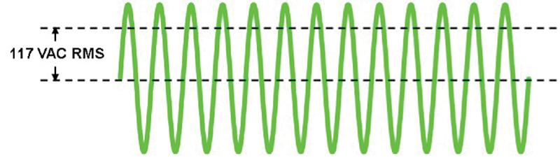
The voltage or current of an AC waveform is usually expressed as an RMS value. For instance, the electricity from a North American household electrical outlet is a low frequency (60 hertz) sine wave whose RMS voltage is about 117 VAC. See Figure 6.

An unmodulated sinusoidal RF signal is an AC waveform, too, but typically with a frequency measured in kilohertz (kHz), megahertz (MHz), or even higher. The amplitude of an RF signal also can be expressed in a variety of ways: voltage (volts), current (amperes) or power (watts). But our field meters and other instruments generally don’t report RF signal level using those metrics. So how do we characterize signal level?

Let’s look at some examples RF signal voltages at various locations in a cable network. As you might expect, per-channel signal voltages in a 75 ohms impedance cable network can vary over a considerable range of values:

• Line extender input: 10 millivolts (mV) root mean square (RMS)

• Line extender output: 100 mV RMS

• Tap spigot output: 7.08 mV RMS

• Set-top input: 1 mV RMS

The decibel and dBmV

A convenient way to deal with the wide variety of signal levels is to use the decibel (dB).

A signal level in millivolts can be expressed in decibels as a ratio of that signal level to a “zero” reference of 1 mV in a 75 ohms impedance, which we call decibel millivolt, or dBmV. ^[1] That reference is 0 dBmV, or (0.001 volt)²/75 ohms = 13.33 nanowatts. This relationship forms the basis for the decibel millivolt (dBmV), which is technically a unit of power expressed in terms of voltage. Mathematically, when the impedance is 75 ohms, dBmV = 20log₁₀(value in millivolts/1 mV).

For example, what is 10 mV RMS in dBmV?

dBmV = 20log₁₀(10 mV/1 mV)

dBmV = 20 * log₁₀(10)

dBmV = 20 * 1

dBmV = 20

After converting to dBmV, the previous signal level examples become:

• Line extender input: 10 mV RMS = +20 dBmV

• Line extender output: 100 mV RMS = +40 dBmV

• Tap spigot output: 7.08 mV RMS = +17 dBmV

• Set-top input: 1 mV RMS = 0 dBmV

For more on decibels, see “The Wise and Mighty Decibel” in the Summer 2017 issue of Broadband Library, available online at https://broadbandlibrary.com/wise-and-mighty-decibel/. Another helpful resource is SCTE 270 2021 Mathematics of Cable (https://www.scte.org/standards/library/catalog/scte-270-mathematics-of-cable/).

What happens when the RF carrier is, say, amplitude modulated? Where in the varying amplitude signal shown in Figure 7 do we measure the signal level?

 

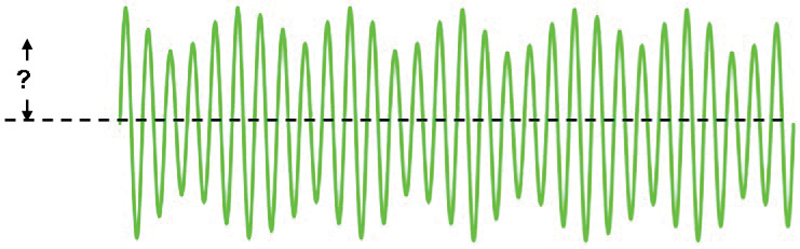
One approach is to measure peak envelope power (PEP), where PEP is the average power (watts) during one cycle at the crest of the modulation envelope.

Start with peak envelope voltage (PEV) — for this example let’s assume the PEV is 14.14 mV, as shown in Figure 8.

 

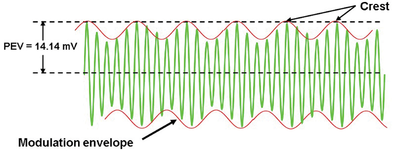
PEP = (PEV * 0.707)²/R

PEP = (0.01414 volt * 0.707)²/75 ohms

PEP = (0.01)²/75

PEP = 0.0001/75

PEP = 1.33 * 10^-6 watt, (0.00000133 watt, or 1.33 µW), during each cycle at the crest of the modulation envelope.

It would be quite cumbersome to express cable network signal levels in PEP — as in “the line extender’s per-channel input signal level is 0.00000133 watt PEP.” As previously mentioned, PEP is the average power of one cycle during the crest of the modulation envelope, which, in the case of an analog National Television System Committee (NTSC) television signal’s visual carrier, occurs during the sync pulses.

The sync pulses represent the carrier’s maximum power; the sync pulses have a constant amplitude even as picture content varies.

Assuming 75 ohms impedance, 0.00000133 watt is 10 mV RMS, or +20 dBmV. Here, +20 dBmV is the RMS value of the instantaneous sync peaks — a unit of power (0.00000133 watt PEP) expressed in terms of voltage (10 mV RMS).

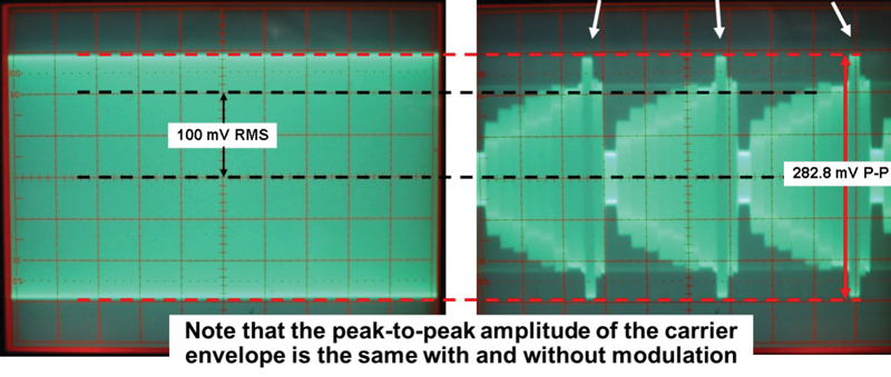
The unmodulated analog TV signal’s visual carrier amplitude in the left screen shot in Figure 9 is 100 mV RMS, or +40 dBmV. When video modulation is applied, the carrier’s amplitude is measured just during the sync peaks (arrows in right screen shot). Here, too, the level is 100 mV RMS, or +40 dBmV.

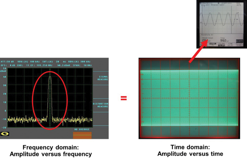
The previous example is a measurement in the time domain; the screen shots were taken from an oscilloscope display. The screen shots in Figure 10 show a frequency domain representation of an unmodulated carrier as seen on a spectrum analyzer (left image), and the same signal as seen in the time domain on an oscilloscope (right photo). The smaller inset screen shot in the upper right also is from an oscilloscope display, but with the time-per-division control adjusted to show a close-up of a sine wave.

What about SC-QAM signals?

As just discussed, the level of an analog TV signal is the PEP of its visual carrier.

When measuring the level of a single carrier quadrature amplitude modulation (SC-QAM) signal, we measure that signal’s average power (not its PEP), also called digital channel power or digital signal power.

Most digital-capable signal level meters, QAM analyzers, and similar test equipment measure the level at several points across an SC-QAM signal’s occupied bandwidth — say, 6 MHz — then integrate the results to provide the average power of the entire “haystack.” Results are typically comparable to what a thermocouple power meter would measure.

The screen shot on the left in Figure 11 shows a frequency domain representation

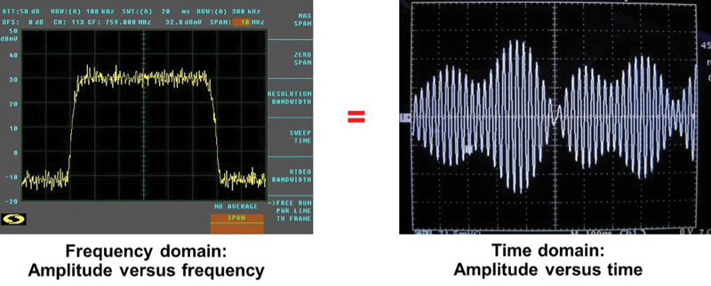
of a 64-QAM signal as seen on a spectrum analyzer, and the right screen shot is the same signal as seen in the time domain on an oscilloscope.

Wrapping up the basics

When we measure the level of an analog TV signal’s visual carrier, we are measuring its peak envelope power. For a legacy SC-QAM signal, we measure the entire haystack’s average power. And for orthogonal frequency division multiplexing (OFDM) signals, we also measure average power.^[2] Signal level measurement results can certainly be expressed in watts or even volts, but those values tend to be pretty cumbersome. Use of the decibel in the form of dBmV provides a handy way of stating signal level relative to a specified reference. Assuming an impedance of 75 ohms, 0 dBmV equals 1 mV, or 13.33 nW.

So, what is signal level? It’s the power of a signal, stated in dBmV, which is technically a unit of power expressed in terms of voltage. Measuring signal level in a cable network is relatively straightforward, and modern test equipment simplifies the task of accurate measurement of analog TV signals, SC-QAM signals, and even OFDM signals.

[1] In Europe and elsewhere, the decibel microvolt (dBμV) is used instead of dBmV for cable network signal level measurements. In this case, the “zero” reference is 1 microvolt (μV) in a 75 ohms impedance, or 0 dBμV, which equals 13.33 femtowatts. Converting between dBmV and dBμV is fairly easy, requiring only subtraction or addition of 60. For example, 0 dBμV = -60 dBmV, and 0 dBmV = +60 dBμV.

[2] From SCTE 270 2021, the average RF power of an OFDM signal is usually characterized in two ways: (1) OFDM power per CTA channel — that is, the average power per 6 MHz (which may not be uniform across the OFDM signal because of exclusion bands and other factors). Also called OFDM channel power. (2) OFDM total power: The average power over the entire occupied bandwidth of the OFDM signal, defined mathematically as total power = Power per CTA channel + 10log₁₀ (number of CTA channels occupied by the OFDM signal).