Basic HFC AC Design (Part Two)
By H. Mark Bowers
In Part One of this article that appeared in the Summer 2018 issue of the Broadband Library we reviewed basic AC network design principles. We then continued with sample calculations for linear-mode power packs, which draw a constant current within a specified voltage range. While this makes for a simplified approach to the calculations, it doesn’t represent ‘real world’ AC powering in the modern cable network. That’s because today’s cable television network actives (and almost all modern electronic devices with a power supply) employ switch-mode circuitry. Switch-mode designs consume a constant power within a stated voltage range; therefore, as the voltage decreases they draw an increasing amount of current. If you are preparing to read this article but have not read Part One in the Summer issue, I recommend that you do so before proceeding.
Amplifier Tree or Nodal Layout: Preparation for AC design calculations requires a diagram of all amplifiers (system actives) in a tree-branch configuration as was shown in Part One of this series. A more detailed diagram is now shown in Diagram One.
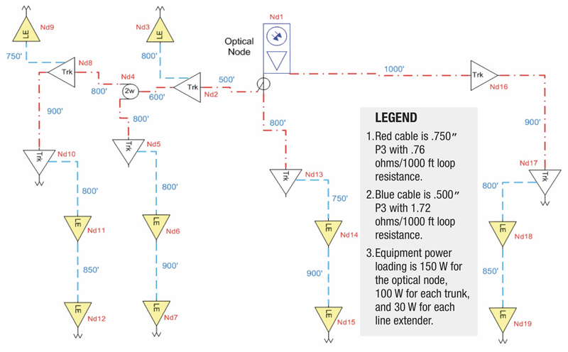
The nodal diagram should contain the following basic information:
- Cable size(s), loop resistance(s), distance(s) between cable ‘breaks,’ and equipment loading in watts (or current in amperes for linear mode) are required (and shown in the legend in Diagram One).
- As implied previously, the location of all current dividing paths, i.e., splitters, directional couplers, amplifiers, etc. In other words, any location where the current can route in different directions.
- Optional: the location of any point in the network where you suspect you may wish to place an AC supply, either now or in the future.
- Assignment of reference nodal numbers on the tree diagram. Assuming you have access to a more sophisticated approach such as a computer design program, a nodal layout is usually necessary to enter and calculate your design.
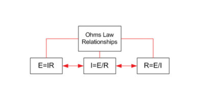
Basic Current and Power Calculations: In review, if the AC current rating of the equipment is used, computations will employ typical voltage drop calculations. Resistance values are calculated for each section of cable. Current draws are known for each device in the network that must be powered. Voltage drops for each section of cable are then computed using the Ohms Law formula V=IR. Be sure to include all currents passing through each section of cable when calculating the voltage drop. For example, if a section of cable has a total resistance of 4 ohms, and has a current of 2 amperes (.25 A for the local device and 1.75 A for downstream devices) flowing through it, the voltage drop for the preceding cable section is 8 volts. Once voltage drops for each plant area are known, you can start at the supply and sum voltage drops to arrive at specific load voltages at each device. This voltage should not drop below manufacturers recommendations for a given device.
If the AC power in watts of each active is employed, an iterative calculation technique must be employed that approximates the following algorithm:
- The initial current draw at the supply voltage (60 or 87 volts) is calculated for each device. The formula to calculate current draw will ideally include the efficiency of the switch-mode circuitry.
- The approximate voltage at each nodal location is then calculated given the current loading on all cable lines.
- The current draw of each device is then re-calculated using the adjusted voltage at each nodal location given preceding voltage drops in the network. Remember, the current draw of a switching regulated device is inversely proportional to the voltage supplied.
- The previous step is repeated multiple times until {the} voltages calculated on successive iterations at each device do not vary by more than a very small value.
- Design results are then displayed.
Obviously a computer program is needed for this iterative approach. And this method, when properly applied, yields very accurate results.
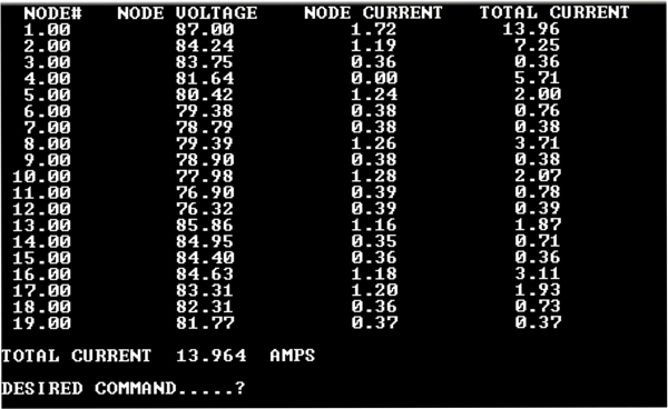
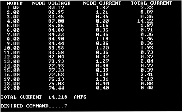
Complete Calculations: Diagram Two shows final calculated voltages and currents if an 87 VAC power supply is placed at nodal location #1 in Diagram One. Minimum voltage at any nodal point was specified at 50 VAC and total power supply loading at ≤ 14 amperes. Therefore, this design is acceptable; but, is there a more optimal location? Remember, with switch-mode power packs higher average network voltages means reduced total current loading on the main supply.
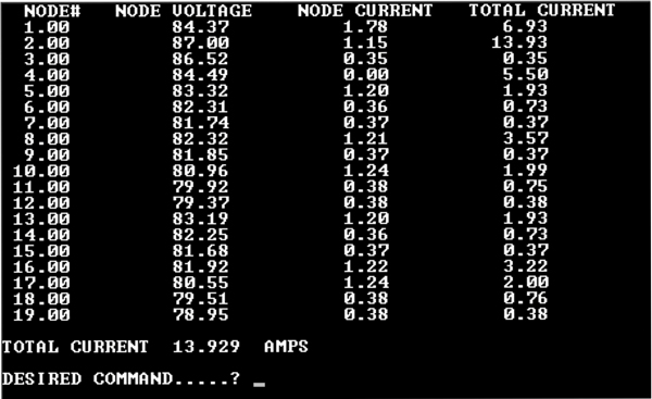
The results in Diagram Three illustrate voltages and currents if the main power supply were moved to nodal location #2. Network voltages, on average, are slightly higher and the total main supply load is reduced by .04 amperes. So this location is slightly improved from nodal location #1.
Finally, let’s check our results if we move the main power supply to nodal location #4. In Diagram Four, total supply loading is approximately .4 amperes higher as compared to nodal location #2. So, we are clearly moving away from the optimal location. However note that this location, although not optimal, will work if it was our only choice for supply placement and if we are willing to allow supply loading to exceed 14 amperes.
Several conclusions can be drawn from these three powering runs.
- We are in the correct general areafor optimal power supply placement.
- We have some flexibility in where we place the supply, i.e., anywhere between nodal locations #1 and #4 will work, with somewhere close to nodal location #2 as the optimal location.
And in case you are wondering whether 60 VAC power would work in this fictitious optical node area, the calculated results of a 60 VAC powering run with the main power supply at nodal location #2 yield a total supply loading of 21.8 amperes and node AC voltages as low as 47 VAC. Worse, the current draw on one side of the power inserter was almost 11 amperes, and many inserters won’t handle that much current on an output leg. Therefore, if 60 VAC were employed, two plant power supplies will be required for this optical node.
Precautions:(“Why aren’t my calculations closer to measured field values?”)Measured system voltages and currents often vary from calculated values for several reasons. Reasons for these variations are:
- Equipment manufacturers often publish current and/or power specifications for their equipment that are worst-case rather than nominal.
- Many designers use fully loaded amplifier station power ratings, even though the system may not fully load their stations.
- Actual network footages are often less than those indicated on system maps. This can occur for a variety of reasons, not the least of which is a common practice during strand or as-built mapping of slightly over estimating footages. For example, the field measurement between a pole and pedestal is 102 feet, however the walk-out person records 105 or even 110 feet. The cumulative effect of this practice impacts the accuracy of the calculations.
- Actual cable “loop resistance” values are sometimes less than the cable manufacturer’s published values, and they are usually specified at a specific temperature, often 68 deg F. As temperature increases so does loop resistance. Significant swings in temperature can create significant changes in voltages and currents in aerial plant under certain conditions.
All of the previous often acts to create ‘head room’ in the AC design, which can be desirable as long as the variance is not too great.
Conclusion
I want to close Part Two with an anecdotal story that illustrates how AC designs with switch-mode power packs, which are desirable because they are very efficient, can introduce complexities and odd behavior if not accomplished properly.
Years ago I was contacted by a major cable operator to help resolve an unusual powering problem in several systems in Ohio. My primary role was to arbitrate meetings among the operator, the amplifier manufacturer, and the mainline power supply manufacturer, because the situation had deteriorated to the point that they were not working well with each other. The symptoms were as follows. During the colder months of the year everything seemed to work correctly, i.e., no powering problems were evident. However, during the heat of summer the system sometimes suffered major outages by power supply area, almost as if the AC power was turned off for several minutes and then came back on. If you consider our switch-mode calculations, as we move the mainline supply to different locations we saw how the total current loading increased or decreased. This implies the following scenario can occur.
If the original design has very little headroom (or has been extended without consideration of the additional powering load), it may just barely work in colder temperatures (with lowered loop resistance in aerial plant), but in the heat of summer the following can occur.
- As the ambient temperature slowly increases, so does loop resistance and the voltage drops throughout the network.
- With switch-mode supplies, the decrease in voltage at each active results in increased current draw at each active, which then increases distributed voltage drops even further.
- The result is an escalating current draw at plant extremities, and when ambient temperature reaches a certain level this creates a ‘cliff effect.’ Currents increase rapidly until fuses blow, breakers trip, or the saturated windings on the ferro-resonant supply simply collapse.
Field measurements on several afternoons using a voltmeter and clamp-on amprobe (at multiple locations), along with a review of their node power designs confirmed that this was indeed their issue. Since the original system design employed 60 VAC powering, the simplest and least expensive solution was to change plant powering to 87 VAC and their problems were resolved. What was originally thought to be a major flaw in power supply or amplifier power pack design turned out to be poor AC network design.
 H. Mark Bowers,
Cablesoft Engineering, Inc.
Mark is VP of Engineering at Cablesoft Engineering, Inc. He has been involved in telephony since 1968 and the cable industry since 1973. His last industry position was VP of Corporate Engineering for Warner Cable Communications in Dublin, OH. Mark’s education includes the U.S. Naval Nuclear Engineering School, and BS and MS Degrees in Management of Technology. Mark is a member of the SCTE, the IEEE, and is a Senior Member and licensed Master Telecommunications Engineer with iNARTE.
Credit: Charts provided by author