Two-way Splitters: A Peek Under the Hood
By Ron Hranac
Two-way splitters have been used by the cable industry for decades. Those simple passive devices can be found on towers, in headends, hubs, the outside distribution network, and the subscriber drop. They’re part of the circuitry inside of some distribution passives such as taps and even other splitters! For example, a four-way splitter comprises a two-way splitter feeding a pair of two-way splitters. If you’ve ever wondered just how a two-way splitter works, grab a cup of coffee and read along!
A splitter is a power divider. In the case of a balanced two-way splitter (more on “balanced” in a moment), when a radio frequency (RF) signal is applied to a splitter’s input port (Port 1 in Figure 1), the signal appears at equal amplitudes and with the same phase at each of the two output ports (Ports 2 and 3 in Figure 1). However, the RF power level at each output port is approximately half of what it was at the input port.
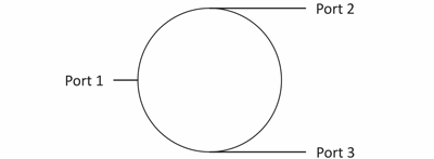
Figure 1. Two-way splitter symbol.
As well, a two-way splitter can be a power combiner. In this usage, what were previously the splitter’s two output ports are now input ports, and the original input port is now the output port. Here, RF signals from two sources can be applied to the two input ports (Ports 2 and 3 in Figure 1), and will appear at the single output port (Port 1 in Figure 1). There is some “it depends” when it comes to the combined power, though. To get you thinking about that, consider the pair of back-to-back two-way splitters connected as shown in Figure 2. What’s the end-to-end insertion loss of this pair of splitters from input port to input port? The answer is at the end of the article.
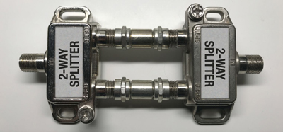
Figure 2. What is the total end-to-end insertion loss through these two combined splitters?
Before moving on, let’s take a quick look at definitions of some other common terminology applicable to splitters in general.
Additional (or excess) insertion loss— Real-world splitters have somewhat higher insertion loss than what is calculated with the formula in the definition for “Insertion loss.” That additional or excess insertion loss is on the order of 0.5 dB to 1 dB (for a total insertion loss of 3.5 dB to 4 dB in a two-way splitter), and is caused by losses in the splitter’s internal transformers’ ferrite-core material and their very small gauge wire windings.
Balanced splitter— A multiple-output splitter that has equal insertion loss or attenuation between the input port and each of the output ports.
Flatness— A measure, in decibels, of amplitude-versus-frequency within the splitter’s passband. Flatness can be degraded if unused ports are left unterminated.
Insertion loss— A reduction of RF power, expressed in decibels, between a splitter’s input port and each of its output ports (see Figure 3). For a balanced splitter, the theoretical insertion loss is defined mathematically as LdB= 10log10(N), where LdBis the loss in decibels, and N is the number of output ports. For example, a balanced two-way splitter has 10log10(2) = 3.01 dB of insertion loss between the input port and each output port, and a four-way splitter has 10log10(4) = 6.02 dB of insertion loss between the input port and each output port.
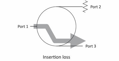
Figure 3. A splitter’s insertion loss is measured between the input port and each of the output ports (with unused ports terminated).
Isolation— A measure of the attenuation of RF power between any two of a splitter’s output ports, when all other ports are properly terminated in the splitter’s characteristic impedance. See Figure 4.
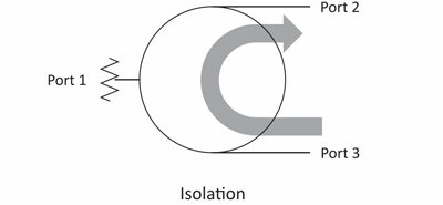
Figure 4. Splitter isolation is measured between any two of a splitter’s output ports, with all other ports terminated.
Passband— The specified operating frequency range of a splitter — for example, 5 MHz to 1002 MHz — over which the insertion loss is approximately equal at all frequencies. While splitters are generally considered to be flat-loss devices, in reality there is slightly more loss at higher frequencies than at lower frequencies.
Unbalanced splitter— A multiple-output splitter that has unequal insertion loss or attenuation between the input port and each of the output ports.
Let’s go back to the concept of a two-way splitter as a power divider. Why not just use a simple tee or twist the conductors of three cables together as shown in Figure 5? After all, won’t that divide the power more or less equally between the two outputs? Yes, but…
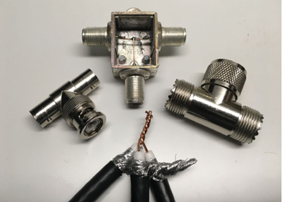
Figure 5. A simple tee or even cable conductors twisted together will function as a splitter, but with significant limitations (see text).
If we assume that the impedance of the loads connected to each of the tee’s two outputs is 75 Ω, the input signal will “see” an impedance of 75/2 = 37.5 Ω. That impedance mismatch is definitely not desirable in a 75 Ω impedance network, and the port-to-port isolation will depend upon the impedance “seen” at the input port. If the input port is terminated in 75 Ω, the tee’s isolation will be about 3 dB. If the input port is an open circuit, the isolation will be 0 dB. In the case of the three cables with their conductors twisted together (and the splitter-without-a cover-turned-into-a-tee), signal leakage and ingress are additional concerns.
To overcome the impedance mismatch that occurs when using a simple tee, the splitter needs some kind of impedance matching circuit.
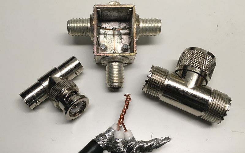
Looking at the schematic and photo in Figure 6, T1 is a ferrite-core autotransformer that functions as a 2:1 impedance matching transformer; the tap is at the 37.5 Ω impedance point. Now the two-way splitter’s 75 Ω input impedance is properly matched to the internal impedance mismatch (37.5 Ω) caused by the split itself. (Note: An autotransformer is a transformer that has only one winding, parts of which function as both primary and secondary windings.)
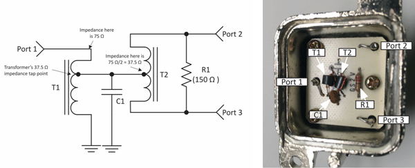
Figure 6. Basic two-way splitter schematic (left) and the inside of a drop splitter with the components marked (right). Assume that all ports are terminated in 75 Ω.
What about isolation? That is achieved with the combination of transformer T2 (150 Ω end-to-end impedance) and resistor R1 (150 Ω). T2 is a center-tapped ferrite-core autotransformer with a 2:1 turns ratio, whose end-to-end impedance is 4x the 37.5 Ω impedance from the center tap to either end. If a signal is injected into one of the output ports (Port 2 or 3 in Figure 6), equal currents flow through T2 (with a 180° phase shift) and R1 (no phase shift), cancelling each other and providing high isolation between Ports 2 and 3.
T1 and the T2/R1 combination are interconnected as shown in Figure 6; capacitor C1 helps improve the overall return loss (impedance match). Since the T2/R1 “tee” has inherently high isolation by itself, the impedance seen at the splitter’s input port (Port 1) will now be the major factor affecting isolation. If Port 1 “sees” 75 Ω, the splitter isolation will be maximum, with real-world values in the 20 dB to 30 dB (or somewhat higher) range. An open or short circuit at Port 1 will reduce the isolation between Ports 2 and 3 to about 6 dB.
Modern “digital ready” drop splitters usually include additional components not shown in Figure 6, which help to reduce the susceptibility to being overdriven by high RF levels (think cable modem upstream signals). Several years ago a phenomenon called passive device intermodulation was discovered to be a problem, where high RF levels could saturate the splitter’s ferrites and cause them to generate intermodulation distortion.
Splitters that are used in the hardline distribution network also include additional components, which are used to accommodate passing 60 to 90 volts for powering plant actives.
Some drop-type splitters — especially those used in residential satellite installations — are designed to pass electrical current between, say, a satellite receiver and the antenna’s low noise block converter (LNB).
Modern splitters are designed to have good RF shielding performance to avoid leakage and ingress problems, a wider passband (1 GHz or more), and high return loss on each port (see the Spring 2017 issue of Broadband Libraryfor more information on return loss: https://broadbandlibrary.com/return-loss/).
As you can see, the seemingly simple two-way splitter has a lot going on under the hood!
Now, what about the insertion loss of the two back-to-back splitters in Figure 2? At first glance you might be inclined to think the answer is 7 dB. After all, each splitter’s nominal insertion loss is about 3.5 dB, so two splitters in series as shown should total 7 dB, right? Nope. The answer is about 1 dB. Here’s why: The RF signal power at each of the two outputs of the first splitter is attenuated by ~3.5 dB, as expected. However, when combined through the second splitter, the signals add because they are in-phase. If the splitters were perfect, there would be no insertion loss through the combined pair because of the in-phase splitting and combining, but there is about 0.5 dB of additional (or excess) insertion loss per splitter, so the total loss is ~1 dB.
References
“Understanding Power Splitters,” Mini-Circuits AN10-006
Ciciora, Walter, J. Farmer, D. Large, M. Adams; Modern Cable Television Technology, 2nd Edition, ©2004, Morgan Kaufmann Publishers (Chapter 10, “Coaxial RF Technology”)
Grant, William; Cable Television, Third Edition, ©1998, GWG Associates (Chapter 3, “Introduction to Equipment”)
 Ron Hranac
Technical Marketing Engineer,
Cisco Systems
Ron Hranac, a 46-year veteran of the cable industry, is TME for Cisco’s Cable Access Business Unit. A Fellow Member of SCTE, Ron was inducted into the Society’s Hall of Fame in 2010, is a co-recipient of the Chairman’s Award, an SCTE Member of the Year, and is a member of the Cable TV Pioneers Class of ’97. He received the Society’s Excellence in Standards award at Cable-Tec Expo 2016. He has published hundreds of articles and papers, and has been a speaker at numerous international, national, regional, and local conferences and seminars.