Why 75 Ohms?
Most modern cable networks are constructed using a combination of optical fiber and coaxial cable technology. The coaxial cable portion of the network—including the antenna site, headend, hub sites, hardline distribution plant, and subscriber drops—uses cables with a characteristic impedance of 75 ohms (Ω). But why 75 Ω? Before attempting to answer that question, it will be helpful to define characteristic impedance.
Characteristic impedance in coaxial cable
A property of a transmission line such as coaxial cable, called characteristic impedance, Zc (sometimes Z0), is equal to the ratio of voltage E to current I in a traveling wave propagating along that transmission line: Zc = E/I.
It’s important to note that the above ratio applies to a traveling wave, not a standing wave (the latter caused by a superposition of two traveling waves propagating in opposite directions along the transmission line—one an incident wave, the other a reflected wave).
In an ideal lossless transmission line such as coaxial cable, the voltage E and current I that occur as a result of the traveling wave are exactly in phase. In real-world coaxial cable, the surfaces of the conductors are not perfectly smooth, and have tiny, even microscopic, imperfections that can affect the cable’s performance. The conductivities of the conductors—the center conductor and shield—are finite, and the flow of RF current “penetrates” the surface of the conductors somewhat. For more about skin effect and skin depth, see SCTE 293-6 2024, What is … Skin Effect and Skin Depth?, available on SCTE’s standards download page (https://account.scte.org/standards/library/catalog/).
The electromagnetic field traveling in the dielectric also penetrates slightly into the conductors. As a result, the conductor loss causes the phase of the electric field to lag slightly behind the phase of the magnetic field, which in turn causes a small capacitive reactance in the cable’s characteristic impedance. For more about this phenomenon, see Handbook of Coaxial Microwave Measurements, originally published by GenRad, Inc., and reprinted by Gilbert Engineering (now Corning-Gilbert). This publication is, unfortunately, out of print, but pdf copies can sometimes be found online.
A transmission line’s characteristic impedance is sometimes called surge impedance, and is related to the transmission line’s inductance L per unit length and capacitance C per unit length. In an ideal lossless transmission line, the characteristic impedance is Zc = √(L/C).
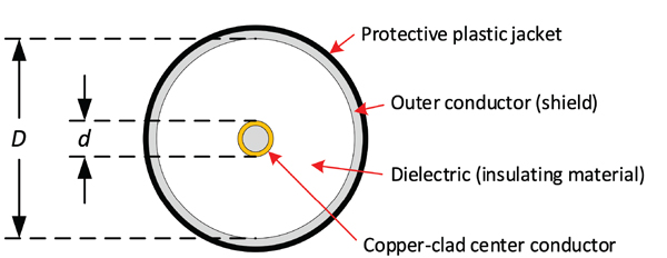
For coaxial cable, the characteristic impedance is related to the ratio of the inside diameter D of the shield to the outside diameter d of the center conductor (and the dielectric constant); see Figure 1.
.
The characteristic impedance of lossless coaxial cable with a perfectly smooth center conductor and shield is Zc = (138/√ε) × log10(D/d)
where
Zc is the coaxial cable’s characteristic impedance in ohms
ε is the dielectric constant
D is the inside diameter of the shield
d is the outside diameter of the center conductor
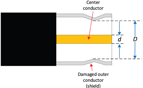
From the above, as long as the ratio of D to d remains constant (and the dielectric constant does not change), the size of the coaxial cable does not affect its characteristic impedance. That’s why 0.500 inch diameter hardline cable has the same 75 Ω characteristic impedance as 0.750 inch diameter hardline cable, assuming both have the same dielectric constant. That relationship also shows why a kink in the cable will cause an impedance mismatch, because the ratio of D to d at the location of the kink is different than the undamaged part of the cable. See Figure 2.
.
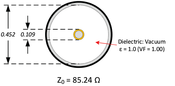
The presence of dielectric material between the center conductor and shield will reduce the characteristic impedance compared to no dielectric material. Here’s an example. Assume a 0.500 inch diameter hardline cable with a vacuum between the center conductor and shield, as shown in Figure 3.
.
Given the values of d = 0.109 inch and D = 0.452 inch, and a vacuum between the two conductors (ε = 1.0), the calculated characteristic impedance is 85.24 Ω.
Adding a dielectric material between the conductors that has a dielectric constant ε = 1.32, the calculated characteristic impedance is 74.16 Ω, as illustrated in Figure 4
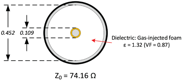
Note: Coaxial cable published specifications generally do not include the dielectric constant. Most published specifications do, however, include the cable’s velocity factor (velocity of propagation in decimal form), from which one can calculate dielectric constant using the formula ε = 1/(VF)2. For the example shown in Figure 4, the cable’s VF is 0.87, which is the same as 87% velocity of propagation.
The dielectric constant itself also affects the cable’s characteristic impedance. For fixed conductor dimensions, varying a cable’s dielectric constant will change the characteristic impedance. If the dielectric constant of an existing dielectric material is changed for whatever reason, the cable’s characteristic impedance will also change. For instance, the presence of water in a coaxial cable’s foam dielectric will change the dielectric constant, causing the cable’s characteristic impedance to change, degrading the performance of that cable.
An important point: Characteristic impedance should not be confused with electrical impedance. Impedance in an electric circuit can change with frequency, but generally speaking, the characteristic impedance of coaxial cable within the radio frequency (RF) range we use in our networks does not change significantly as long as the dielectric constant does not vary, and the ratio of the inside diameter of the shield to the outside diameter of the center conductor remains constant. Electrical impedance is a topic for another day.
Okay, why 75 Ω?
The introduction to this article states “The coaxial cable portion of the network … uses cables with a characteristic impedance of 75 ohms (Ω).” One question that comes up from time to time is why 75 Ω and not, say, 50 Ω? After all, 50 Ω characteristic impedance cables have long been used in broadcasting and radio communications. Let’s look at some of the reasons that might provide an answer.
Availability of surplus coaxial cable
One of the most common reasons I’ve heard over the years is the widespread availability of military surplus 75 Ω characteristic impedance coaxial cable after the end of World War II. Many early cable systems were built using some of that surplus cable.
Coaxial cable attenuation-versus-impedance
Another reason given is related to the attenuation of 75 Ω characteristic impedance coaxial cables of a given size compared to cables of the same physical size with other impedances. This goes back to research conducted by Lloyd Espenscheid and Herman Affel of Bell Telephone Laboratories in the late 1920s and early ’30s. The two were working on solutions to transport 4 MHz signals long distances using coaxial cable, the latter patented by the pair in 1929 (the patent was granted in 1931). For air dielectric coaxial cables, the best attenuation-versus-impedance was found to occur at about 77 Ω impedance; the maximum peak power handling at about 30 Ω; and the maximum voltage at about 60 Ω.
Before the widespread adoption of optical fiber technology and the birth of what is now known as hybrid fiber/coax (HFC) network architectures, many cable networks had lengthy trunk amplifier cascades (in the late 1970s I worked in a system that had a 67 amplifier cascade). The use of lower attenuation coaxial cable meant somewhat fewer amplifiers in those trunk cascades, hence the reasoning for 75 Ω characteristic impedance cables instead of some other impedance.
Ease of impedance matching to TV tuner
One possible reason for the use and availability of 75 Ω characteristic impedance coax in cable TV applications was the ease of matching the coaxial cable’s impedance to that of the 300 Ω impedance of older analog TV tuners. A relatively simple 4:1 balun (2:1 turns ratio) converted between the tuner’s 300 Ω (balanced) input and the 75 Ω impedance (unbalanced) coaxial cable. This reason seems highly unlikely and a bit of a stretch, given that designing and manufacturing a 6:1 balun (2:45:1 turns ratio) to convert between 300 Ω and 50 Ω could have been done.
Close to impedance of half-wave dipole antenna
Section 10.2.5 of the book Modern Cable Television Technology, 2nd Ed., notes “…the loss minimum is at about 80 ohms, for air dielectric (dielectric constant = 1.0), and decreases as the dielectric constant increases.” That section goes on to state “…75 ohms may have been chosen because it is also close to the feed-point impedance of a half-wave dipole antenna. In order to minimize the need for repeaters, wide area distribution systems universally use 75-ohm cables.”
The book’s discussion about attenuation-versus-impedance is consistent with the results of work by Espenscheid and Affel mentioned previously. It’s more difficult to know for certain whether the availability of 75 Ω coaxial cable is related to a half-wave dipole’s impedance.
The feedpoint complex impedance of a thin, lossless half-wave dipole in free space is Z = 73 + j42.5 Ω, which some simply call 73 Ω. But that scalar value leaves out important information: the complex impedance’s reactance. A dipole’s end-to-end length is typically shortened a few percent from a free space half-wavelength value to achieve resonance, usually defined as a purely resistive feedpoint impedance (that is, with no reactance), or with negligible reactance. Practically speaking, a half-wave dipole’s feedpoint impedance is affected by the antenna’s height above ground, proximity to nearby objects, etc., so the element lengths are often simply adjusted to achieve minimum standing wave ratio (SWR) at the input to a feedline connected to the dipole. All of that said, 75 Ω characteristic impedance coaxial cable is sometimes used to feed half-wave dipole antennas, but 50 Ω impedance coaxial cable is much more commonly used for that purpose (especially in applications such as amateur radio). Balanced feedline such as ladder line or window line is also sometimes used.
Lost to history
The real reason or reasons for the cable industry’s choice and use of 75 Ω impedance coaxial cables (and components) might be lost to history, but almost certainly has at least some relationship to a combination of attenuation-versus-impedance, and the widespread availability of surplus 75 Ω characteristic impedance cables after World War II. Those two make the most sense to me.

Ron Hranac
Technical Editor, Broadband Library
rhranac@aol.com
Ron Hranac, a 53 year veteran of the cable industry, has worked on the operator and vendor side during his career. A Fellow Member of SCTE and co-founder and Assistant Board Member of the organization’s Rocky Mountain Chapter, Ron was inducted into the Society’s Hall of Fame in 2010, is a co-recipient of the Chairman’s Award, an SCTE Member of the Year, and is a member of the Cable TV Pioneers Class of ’97. He received the Society’s Excellence in Standards award at Cable-Tec Expo 2016. He was recipient of the European Society for Broadband Professionals’ 2016 Tom Hall Award for Outstanding Services to Broadband Engineering, and was named winner of the 2017 David Hall Award for Best Presentation. He has published hundreds of articles and papers, and has been a speaker at numerous international, national, regional, and local conferences and seminars.
Images provided by author, Shutterstock