Total Power and Power Spectral Density
By Ron Hranac
Two RF power-related parameters that can cause confusion are total power (also called total composite power) and power spectral density (PSD). Grab a cup of coffee and a scientific calculator. We’re going to look at these two parameters a little more closely.
Quick side note: When we measure RF signal level we are measuring RF power. You might wonder why decibel millivolt (dBmV) is used instead of watt (W) for RF power in cable networks. The first reason is the typical power levels we deal with are very small. For example, 0 dBmV is only 13.33 nanowatts (~13 billionths of a watt!). Working in the world of the decibel (dB) makes dealing with very small and very large numbers much easier. The second reason we use dBmV is because that metric expresses power in terms of voltage. For more on the latter, see my Summer 2017 Broadband Library article “The Wise and Mighty Decibel,” available on-line at https://broadbandlibrary.com/wise-and-mighty-decibel/
Total power
As I noted in the Summer 2017 article, “Total power is the combined power of all signals in a given frequency range — for instance, the downstream. It’s of concern because excessive total power is what overdrives lasers, set-tops, modems, and other devices.”
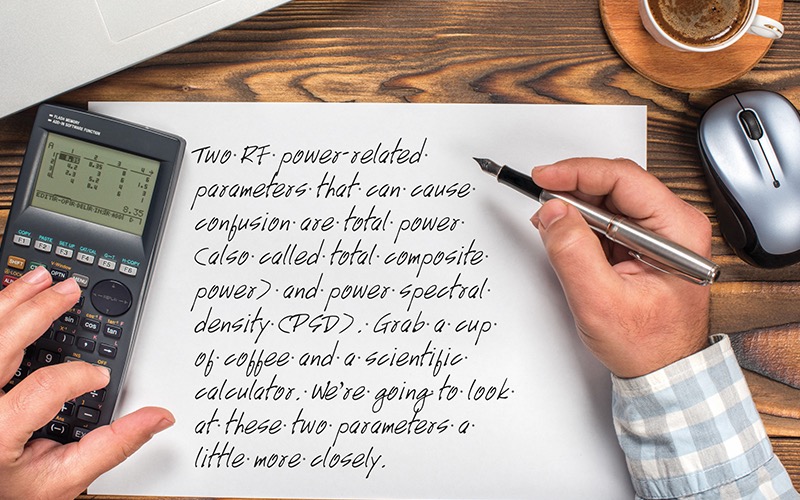
Calculating total power does require some number crunching, since you can’t simply add the individual signal levels in dBmV to get total power. Consider the example in Figure 1, which shows a single RF signal whose power is +20 dBmV. For this and all subsequent examples, assume the impedance is 75 ohms.
Figure 1. RF signal whose power is +20 dBmV.
Converting +20 dBmV to power in watts is done as follows. First, convert dBmV to voltage (millivolts in this case):
mV = 10(dBmV/20)
mV = 10(20/20)
mV = 101
mV = 10 (which equals 0.010 volt)
Next, convert voltage to watts:
P = E2/R
P = (0.010 volt)2/75 ohms
P = 0.0001/75
P = 0.00000133 watt, or 1.33 microwatt (µW)
Since there is only one signal, the total power is +20 dBmV or 1.33 µW. What happens to the total power if the number of RF signals is increased to four, each at +20 dBmV? Refer to Figure 2.
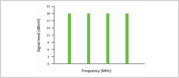
Figure 2. Four RF signals, each with a power of +20 dBmV. What is the total power?
There are a few ways to solve this. The first is to convert the signal level in dBmV to watts, add the watt values, then convert back to dBmV. Since +20 dBmV = 1.33 µW, then 1.33 µW + 1.33 µW + 1.33 µW + 1.33 µW = 5.33 µW (0.00000533 W) total power.
Next, convert watts to voltage:
E2 = PR
E2 = 0.00000533 * 75
E2 = 0.0004
E = 0.02 volt, or 20 mV
Finally convert mV to dBmV:
dBmV = 20log10(mV/1 mV)
dBmV = 20log10(20 mV/1 mV)
dBmV = 20 * [log10(20)]
dBmV = 20 * [1.301]
dBmV = 26.02 dBmV
When all signals have identical power, the following formula can be used to calculate total power: Ptotal = Pone + 10log10(N), where Ptotal is total power, Pone is the power of one signal, and N is the number of signals. For the previous example, Ptotal = 20 dBmV + 10log10(4) = 26.02 dBmV.
Had the four +20 dBmV values simply been added together as is, the resulting +80 dBmV would have been wrong. That’s equal to 1.33 watts!
If the power of each channel is different, a more typical situation, total power is calculated with the formula Ptotal = 10log10[10(P1/10) + 10(P2/10) + 10(P3/10) + … + 10(PN/10) ], where Ptotal is total power in dBmV, and P1, P2, P3…PN are the levels of each channel or signal in dBmV. If you use this formula for the previous example, you’ll get +26.02 dBmV total power.
Ok, go refill that coffee cup. More number crunching is on the way.
Power spectral density
This parameter is a bit trickier to grasp. If you really like gnarly math, see the in-depth article on Wikipedia at https://en.wikipedia.org/wiki/Spectral_density. For the purposes of the discussion here, we can simplify somewhat by saying PSD “describes how power of a signal…is distributed over frequency.” PSD is commonly expressed in power per hertz (Hz).
For the next example (see Figure 3), assume a 1.6 MHz-wide upstream single carrier quadrature amplitude modulation (SC-QAM) signal whose digital channel power is +65 dBmV.
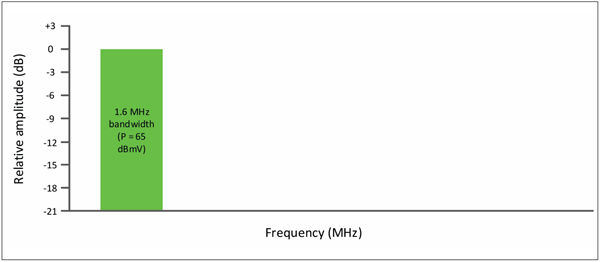
Figure 3. Upstream 1.6 MHz wide SC-QAM signal; P = +65 dBmV.
The PSD is:
PSD = 65 dBmV – 10log10(1,600,000 Hz)
PSD = 65 – [10 * log10(1,600,000)]
PSD = 65 – [10 * (6.20)]
PSD = 65 – [62.04]
PSD = 2.96 dBmV/Hz
Now let’s replace the 1.6 MHz wide signal with one that’s 3.2 MHz wide, but with the same PSD as before (Figure 4). As viewed on a spectrum analyzer, the “haystack” also would be the same height as before. Because the width of the SC-QAM signal is doubled, so is its power. That means the digital channel power is now +68.01 dBmV, a 3.01 dB increase. What about the PSD?
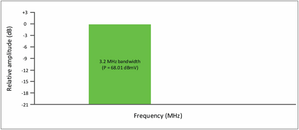
Figure 4. Upstream 3.2 MHz wide SC-QAM signal; P = +68.01 dBmV.
PSD = 68.01 dBmV – 10log10(3,200,000 Hz)
PSD = 68.01 – [10 * log10(3,200,000)]
PSD = 68.01 – [10 * (6.51)]
PSD = 68.01 – [65.05]
PSD = 2.96 dBmV/Hz
Next, replace the 3.2 MHz wide SC-QAM signal with one whose bandwidth is 6.4 MHz. As before, we’re going to maintain the same PSD (same “haystack” height as viewed on a spectrum analyzer), illustrated in Figure 5. Since the bandwidth of the SC-QAM signal doubled again, so did the digital channel power, which is now +71.02 dBmV.
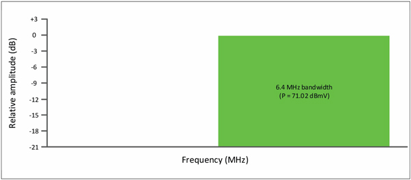
Figure 5. Upstream 6.4 MHz wide SC-QAM signal; P = +71.02 dBmV.
PSD = 71.02 dBmV – 10log10(6,400,000 Hz)
PSD = 71.02 – [10 * log10(6,400,000)]
PSD = 71.02 – [10 * (6.81)]
PSD = 71.02 – [68.06]
PSD = 2.96 dBmV/Hz
Showing all three SC-QAM signals together (Figure 6), we see that they have the same PSD of 2.96 dBmV/Hz and equal haystack heights. The total power is Ptotal = 10log10[10(65/10) + 10(68.01/10) + 10(71.02/10) ] = 73.45 dBmV.
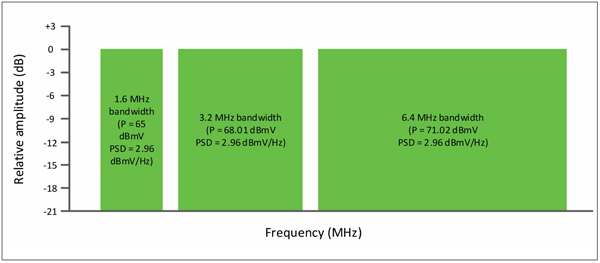
Figure 6. All three upstream SC-QAM signals. PSD = 2.96 dBmV/Hz, and Ptotal = 73.45 dBmV.
Constant power per carrier versus constant PSD per carrier
Most cable modem terminations systems (CMTSs) and cable modems are configured for constant power per carrier in the upstream. In the next two examples, the total power of the four signals is the same (+57 dBmV). Figure 7 shows an example of constant power per carrier, with each SC-QAM signal’s digital channel power equal to about +51 dBmV (+50.98 dBmV). Note that the haystack heights are different for different bandwidth signals, even though each has the same digital channel power. That means the PSD is different for each bandwidth channel: 6.4 MHz channel: -17.08 dBmV/Hz; 3.2 MHz channel: -14.07 dBmV/Hz; and the 1.6 MHz channel: -11.06 dBmV/Hz.
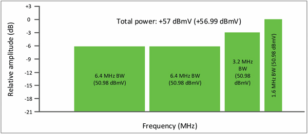
Figure 7. Constant power per carrier. Ptotal = +57 dBmV.
If the four upstream SC-QAM signals were instead set to constant PSD per carrier (-15.46 dBmV/Hz in this example), the spectrum display would look like Figure 8. The haystack heights are the same, but the per-signal digital channel power is different!
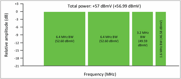
Figure 8. Constant PSD per carrier; Ptotal = +57 dBmV.
Hopefully this exercise helps to clarify total power and power spectral density. I don’t know about you, but my coffee just ran out. That’s enough math for now. Class dismissed!
 Ron Hranac
Technical Marketing Engineer,
Cisco Systems
rhranacj@cisco.com
Ron Hranac, a 46-year veteran of the cable industry, is TME for Cisco’s Cable Access Business Unit. A Fellow Member of SCTE and co-founder and Associate Board Member of the organization’s Rocky Mountain Chapter, Ron was inducted into the Society’s Hall of Fame in 2010, is a co-recipient of the Chairman’s Award, an SCTE Member of the Year, and is a member of the Cable TV Pioneers Class of ’97. He received the Society’s Excellence in Standards award at Cable-Tec Expo 2016. He has published hundreds of articles and papers, and has been a speaker at numerous international, national, regional, and local conferences and seminars.