Getting TDR Functionality on In-Service Cable Lines
By Tom Williams
One of the tough decisions facing line technicians is deciding if suspected line damage is severe enough to warrant taking cable service down to shoot the line with a time domain reflectometer (TDR). This decision is no longer necessary as it is now possible to measure a standing wave on a block of digital signals, and accurately range the distance to a fault on in-service plant using live digital traffic as test signals.
Figure 1 shows the wiring diagram. A non-service interrupting high impedance probe is attached at the output of a tap (or other device) and a spectrum of highly-averaged digital signals is captured as illustrated in Figure 2. The probe can touch, for example, the seizure screw in a tap’s KS port. At a test point that can see signals traveling upstream and downstream, the signals will add in and out of phase at different frequencies, creating a standing wave. By knowing a frequency difference between standing wave peaks, the round-trip time delay can be computed as a reciprocal.
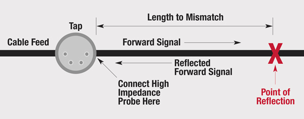
Figure 1. A wiring diagram showing where to insert a high-impedance test probe
Frequency Response with a Single Reflection
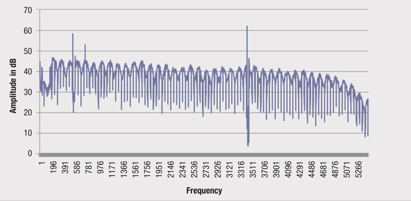
Figure 2. A downstream spectrum containing many digital carriers and a standing wave caused by a reflection
For example, a 1 MHz frequency difference between peaks indicates a 1 microsecond round-trip travel time to the point of reflection and back. Then a distance from the probe to a point of reflection can be computed, assuming you know the cable’s velocity of propagation.
The approximate one-way distance in feet can be calculated with the formula Dft = 492 x (VF/FMHz), where VF is the cable’s velocity factor (velocity of propagation expressed in decimal format) and FMHz is the separation in megahertz between the standing wave peaks. For example, if the frequency spacing between standing wave peaks is the previously mentioned 1 MHz, and the cable’s velocity factor is 0.87, the one-way distance is
Dft = 492 x (0.87/1)
Dft = 492 x (0.87)
Dft = 428
This calculation can be made much more accurately if the frequency response data is plugged into an inverse Fourier transform (IFFT) to produce an impulse response. This can be done with magnitude-only data by (falsely) assuming phase values, such as all zeroes. This creates the time plot of Figure 3 where there are harmonics (H1, H2, etc.) created by the 6 MHz digital channel “haystacks” and the standing wave, indicated by the red arrow. The IFFT can also reveal if there are multiple reflections.
Looking again at Figure 1, if there is only a single point of reflection, the standing wave will not appear at an end point and the response will be flat. This end point could be a cable modem’s (CM) input connector, or an amplifier’s directional coupler test point. This is because the reflected signal will be absorbed, never to be seen again (except by a high impedance probe). If a standing wave is observed at a CM’s input, it can be assumed that there is a second point of reflection responsible for the standing wave. That is, an echo tunnel has been created. While you know accurately a length of the tunnel, you don’t know exactly where in the plant the tunnel is located. Nevertheless, this use case is valuable because most modern CMs have a full band spectrum capture capability, so standing wave data are available to the proactive network maintenance (PNM) management system for analysis, speeding diagnosis and repair.
The harmonics in Figure 3 can be mathematically removed by at least two methods. This can be done by interpolating across the drop-out between 6 MHz QAM haystacks, or by capturing an unimpaired reference forward-only signal and using that as a calibration signal. This forward-only signal can be captured at any one of the amplifier’s four test points.
In conclusion, if you are a tech supervisor, you should not be hearing “We are taking this line down to shoot a TDR response” in the future.
Impulse Response
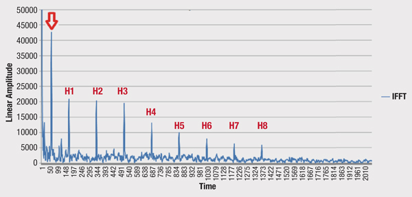
Figure 3. A time response showing the round-trip time from the point of reflection (red arrow). Harmonics are separated by 166.67 ns and are caused by the 6 MHz spacing of downstream QAM channels.
 Tom Williams
Principal Architect, CableLabs
Tom Williams is a Principal Architect with CableLabs. He received his BSEE from Christian Brothers University, his MSEE from the University of Illinois, and his MBA from Eastern Illinois University. He has worked in the Cable industry for 36 years, first at Scientific Atlanta (now Cisco), then at CableLabs, and then as a contractor/consultant, and is currently back with CableLabs. While at CableLabs, Tom has tested digital broadcast signals for compatibility with Cable plant, and evaluated the ability of Cable lines to transport high-speed digital signals. Currently, Tom is working on PHY-layer issues associated with delivery of Gigabit data over cable networks, and advanced network diagnostics. Tom is a prolific inventor with more than 60 patents granted or pending, and enjoys radio frequency (RF) design and digital signal processing (DSP).
CartoonStock.com. Charts provided by author