Reflecting on Impedance Mismatches
An apology for the title, but you’ll get the pun shortly if you haven’t already. I’m pleased to team up with coauthor and long-time friend and industry colleague, Tom Kolze, in this issue of Broadband Library. Tom and I have collaborated on several projects, standards and specifications, documents, and papers over the years.
The coaxial cables in our networks are two-conductor transmission lines that support the propagation of electromagnetic waves, specifically those in the radio frequency (RF) spectrum. A change of the characteristic impedance in a transmission line—for instance, an open circuit, short circuit, or something in between those two extremes—causes a reflection of some or all of the transmitted (incident) RF signal.
Characterizing impedance mismatches
The severity of an impedance mismatch is characterized by a variety of parameters, such as reflection coefficient, return loss, and voltage standing wave ratio (VSWR). Briefly, reflection coefficient is the ratio of reflected voltage to incident voltage, and is commonly represented by the Greek letter gamma (Γ), and sometimes by the Greek letter rho (ρ). The magnitude of reflection coefficient, |Γ|, can have values from 0 (indicating that all the incident energy is absorbed by the load) to 1 (indicating that all the incident energy is reflected by the load). The smaller the magnitude of the reflection coefficient, the more incident energy is absorbed by the load, and this is considered a better “impedance match” than when a larger amount of incident energy is reflected from the load.
Return loss is probably most familiar to cable operators, and is the ratio, in decibels, of the power incident upon an impedance discontinuity to the power reflected by the impedance discontinuity. Return loss can also be described as the difference, in dB, between incident power in dBmV and reflected power, also in dBmV. A larger return loss indicates a better impedance match of the load with the transmission line.
Imagine a continuous wave (CW) carrier transmitted through a length of cable. When the CW carrier reaches an impedance mismatch, some or all of the incident wave is reflected back toward the source. The incident and reflected waves interact to produce a distribution of fields inside the coax known as standing waves. VSWR is the ratio of the maximum peak RF voltage anywhere in the length of cable to the minimum value anywhere along the cable. VSWR is more commonly used in radio communications. VSWR ranges from 1 (sometimes written as 1:1), indicating a perfect impedance match for the load with the transmission line, and no reflected energy from the load, to infinitely large, indicating all the incident energy is reflected back from the load.
For more information about the various ways to characterize the severity of impedance mismatches, see the technical monograph SCTE 293-3 2024 “What is … Return Loss?”, available on SCTE’s standards download page at https://account.scte.org/standards/library/catalog/scte-293-3what-isreturn-loss/
The underlying gremlin in the above is impedance mismatches. Two of those impedance mismatches in a transmission line are analogous to a pair of reflectors.
An example in the outside plant might be two severe kinks in a hardline feeder cable separated by a span or length of that cable. The cable’s impedance is modified at the locations of the two kinks, which can be described as a pair of point impedance discontinuities, as illustrated in Figure 1.
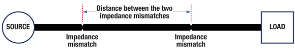
Figure 1. In this example, two severe kinks in the cable change the impedance at the two points, resulting in a pair of impedance mismatches. The impedance mismatches and length between them form a transmission line resonator, more commonly known as an echo tunnel, echo cavity, impedance cavity, or resonant cavity.
What is a transmission line resonator?
That span of cable and the impedance mismatches at each end of the span of cable act as a one-dimensional transmission line resonator, with the resonance frequencies determined by the mismatches’ physical separation distance and the velocity of propagation of the signal through the cable. The velocity of propagation of the signal through the cable is affected by the dielectric constant of the cable. For more information about velocity of propagation and dielectric constant, see the technical monograph SCTE 293-2 2024, “What is … Velocity of Propagation?”, available on SCTE’s standards download page at https://account.scte.org/standards/library/catalog.
Another example of a transmission line resonator is what is called a resonant stub, easily made using a specific length of coaxial cable with either a short circuit or open circuit at one end, and the other end connected in series or parallel with the primary coaxial cable. For instance, one can make a simple notch filter using an electrical quarter wavelength of coax with the far end an open circuit, and the other end connected to a tee in the primary cable. See Figure 2.
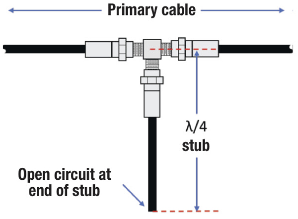
Figure 2. A simple notch filter can be made using an open-circuit electrical quarter wavelength of coaxial cable connected in parallel with the primary cable using a tee.
Getting back to a span of coaxial cable with an impedance mismatch at each end, these transmission line resonators have been more commonly known in the cable industry’s world of proactive network maintenance (PNM) as echo tunnels, echo cavities, impedance cavities, or resonant cavities. While echo tunnels, and echo or impedance cavities are common vernacular in the cable industry, they aren’t exactly the most technically accurate descriptors of a transmission line resonator.
Perhaps surprising to some, transmission line theory doesn’t use the term “echo” in reference to a reflection or reflected wave. “Echo” is usually more applicable to audio, and “impedance cavity” is somewhat vague. Despite being the most technically accurate term, “transmission line resonator” isn’t commonly used in the cable industry.
So, what should we call the span of cable that has an impedance mismatch at each end of the span? Resonant cavity is arguably a good choice. Why? As mentioned earlier, the two impedance mismatches are analogous to a pair of reflectors. The electrical length of the coaxial cable between the reflectors—the two impedance mismatches—forms a resonant circuit of sorts. That resonance shows up in the frequency domain as amplitude ripple. An example of amplitude ripple in a downstream broadband sweep trace is shown in Figure 3.
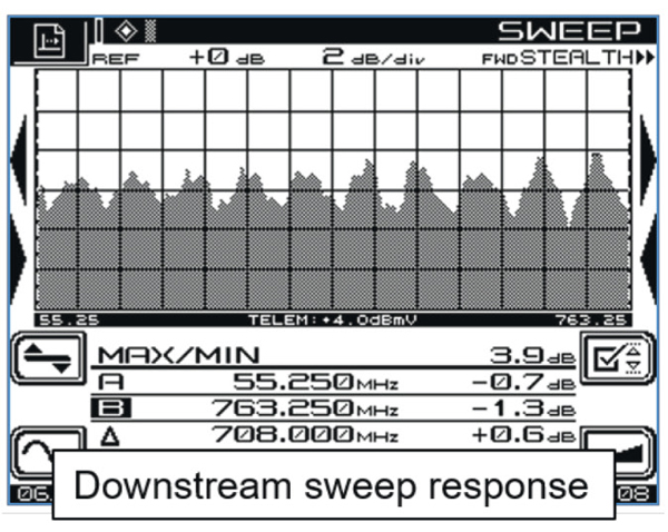
Figure 3. Amplitude ripple on a downstream sweep receiver display.
Knowing the frequency spacing between adjacent peaks or valleys in the amplitude ripple, it’s possible to calculate the distance between the two impedance mismatches—the length of the resonant cavity. Here’s the formula:
Lfeet = 492 × (VF/fMHz)
where
Lfeet is the length of the resonant cavity in feet,
VF is the cable’s velocity factor (velocity of propagation expressed in decimal form), and
fMHz is the spacing in megahertz between adjacent amplitude ripple peaks or valleys.
Example:
Assume a scenario in which two impedance mismatches exist in the outside hardline plant, causing amplitude ripple with 400 kHz spacing. If the cable’s VF is 0.87, what is the length of the resonant cavity? Refer to Figure 4.
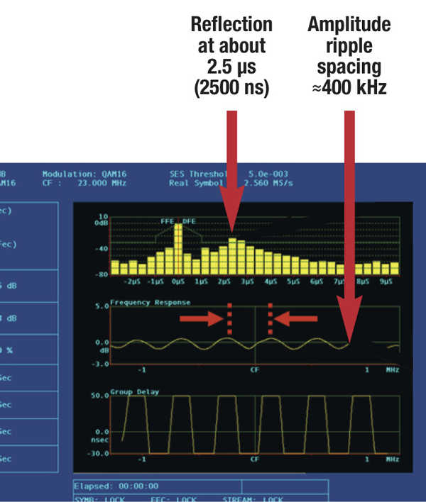
Figure 4. The length of a resonant cavity can be calculated using the amplitude ripple spacing.
Solution:
The resonant cavity length is
Lfeet = 492 × (0.87/0.400 MHz)
Lfeet = 492 × (2.18)
Lfeet = 1070
From this, the length of the resonant cavity is about 1070 feet. You could troubleshoot this in the affected area by looking on system maps for two devices separated by that distance, maybe the output of a line extender and an unterminated end-of-line.
Wrapping up
PNM tools collect data from cable modems and headend/hub equipment such as cable modem termination systems. The tools use that data to help identify the existence of problems or conditions in the outside plant and subscriber drops, the types and severity of problems, and even their locations. A resonant cavity—which goes by a variety of names—is one such condition that can indicate something is amiss, specifically the existence of troublesome impedance mismatches. The terminology we use can sometimes be confusing, especially when trying to describe the effects of those impedance mismatches. Understanding how a pair of them creates a resonant cavity can help to simplify their troubleshooting and repair.
 Ron Hranac
Technical Editor,
Broadband Library
rhranac@aol.com
Ron Hranac, a 52 year veteran of the cable industry, has worked on the operator and vendor side during his career. A Fellow Member of SCTE and co-founder and Assistant Board Member of the organization’s Rocky Mountain Chapter, Ron was inducted into the Society’s Hall of Fame in 2010, is a co-recipient of the Chairman’s Award, an SCTE Member of the Year, and is a member of the Cable TV Pioneers Class of ’97. He received the Society’s Excellence in Standards award at Cable-Tec Expo 2016. He was recipient of the European Society for Broadband Professionals’ 2016 Tom Hall Award for Outstanding Services to Broadband Engineering, and was named winner of the 2017 David Hall Award for Best Presentation. He has published hundreds of articles and papers, and has been a speaker at numerous international, national, regional, and local conferences and seminars.
 Tom Kolze, Ph.D.,
R&D Advanced Technology Development Engineer,
Broadcom, Inc.
Dr. Thomas Kolze was the architect for the DOCSIS® upstream physical layer. He created the flexible physical layer approach for cable upstream transmission, capable of providing good performance to different users with unique channel impairments, and adapting as network conditions change. He is a four-time recipient of the TRW Chairman’s Award for Innovation, inventor on 161 U.S. patents, an IEEE Fellow, and a Cable TV Pioneer. Tom is active in CableLabs and SCTE working groups.
Images provided by authors, Shutterstock