Decibels and Distance

The decibel (dB) has since the beginning of the cable industry been an important part of the foundation of our networks and more. A simple definition of dB is a way to “express the ratio between two power levels.” But what does that have to do with distance?

More formally, from the operational practice SCTE 270 2021r1, Mathematics of Cable (https://account.scte.org/standards/library/catalog/scte-270-mathematics-of-cable/), the decibel is “A logarithmic-based expression of the ratio between two values of a physical quantity, typically power or intensity. The decibel provides an efficient way to express ratios which span one or more powers of the logarithmic base, most commonly 10. Mathematically, the ratio of two power levels P1 and P2 in decibels is dB = 10log10(P1/P2).”

For instance, a 10 watt radio transmitter has 3.01 dB greater power than a 5 watt radio transmitter. Going the other way, a 20,000 watt broadcast transmitter has 3.01 dB less power than a 40,000 watt broadcast transmitter. The absolute difference between two power values isn’t what matters, it’s the ratio between them.

The decibel is commonly used to state parameters such as loss (attenuation), gain, return loss, carrier-to-noise ratio (CNR), carrier-to-distortion ratio (e.g., composite triple beat, or CTB), signal-to-noise ratio (SNR), receive modulation error ratio (RxMER), and more.

With a little mathematical tweaking, we can also use the dB as the basis for radio frequency (RF) signal level in decibel millivolts (dBmV) or decibel microvolts (dBµV), both of which express power in terms of voltage. Another example is power in decibel milliwatts (dBm), used for both RF and optical applications.

For more information, see the technical monograph SCTE 293-1 2024, What is … the Decibel?, available on SCTE’s standards download page at https://account.scte.org/standards/library/catalog/scte-293-1-what-is-the-decibel/. I’ve also written about the good ol’ dB many times over the years, including in the pages of Broadband Library. One example is the article “The Wise and Mighty Decibel” at https://broadbandlibrary.com/wise-and-mighty-decibel/.

Another use for decibels

Did you know that the decibel can be used to state distance? Well, sort of. Here’s a closer look.

Coaxial cable

When I started in the cable industry back in the early 1970s, many networks—including in the system where I worked—had a capacity of just 12 analog TV channels (Ch. 2-13), using an operating bandwidth of 54 MHz to 216 MHz. Cable network architectures were all-coax tree-and-branch, often with relatively lengthy trunk amplifier cascades. Unsurprisingly, this was fairly typical industry-wide in those days. Further, it was common to describe trunk amplifier spacing in dB, based on the loss between amplifiers at the highest downstream frequency ( f_H) or channel. That is still true to some extent today, at least in the case of cascaded actives in node service areas.

Ideally, unity gain was (and still should be) part of cable network design, where amplifier station gain, in dB, is numerically equal to the total loss, in dB, in each cable span between amplifiers. For example, assuming each trunk amplifier in a cascade has 22 dB of gain, maintaining downstream unity gain means the total cable and passive loss in the span immediately upstream of each amplifier should be 22 dB. For more about unity gain, see the technical monograph SCTE 293-5 2024, What is … Unity Gain? at https://account.scte.org/standards/library/catalog/scte-293-5-what-isunity-gain/.

In the days of all-coax tree-and-branch plants it wasn’t unusual for the physical distance between trunk amplifiers to be on the order of 1500 feet to 2000+ ft. If one knows cable and passive loss specifications at the highest downstream frequency, f_H, and the spacing between amplifiers in dB, it’s possible to figure out a physical distance. For the following examples, let’s have a little fun and use typical specs from the late 1960s and early ’70s. I found data for hardline coax from that era in a Jerrold SD-7 Reference Data booklet published in 1967. At the time, both .750 and .500 inch diameter cables were used for trunk applications, and .412 inch diameter coax was commonly used in the feeder.

Let’s use Ch. 13 as the highest downstream channel. That channel’s visual carrier frequency is 211.25 MHz. The Jerrold booklet lists attenuation for JT1500 half-inch diameter coax as 1.32 dB/100 ft. at 211.25 MHz, and 0.96 dB/100 ft. for JT1750 three-quarter-inch diameter coax at the same frequency. (Quick side note: Today’s hardline cables have much better attenuation performance than the older cables did, so don’t try to use these numbers in a modern cable plant.)

For the first example, assume the span between two trunk amplifiers is just coax, as illustrated in Figure 1. To calculate the cable length, use the formula L_feet = (S_dB/L_H) × 100, where L_feet is the length of the coaxial cable in feet; S_dB is amplifier spacing in dB; and L_H is the cable attenuation in dB per 100 feet at the highest downstream frequency f_H.

If the span comprises .500 inch diameter JT1500 hardline coax, and the spacing is 22 dB at f_H = 211.25 MHz, that works out to (22/1.32) × 100 = 1667 feet of coax. For the JT1750 .750 hardline coax, 22 dB of cable at f_H is (22/0.96) ×100 = 2292 feet. Realistically, it’s unlikely an all-coax span between two trunk amplifiers would be the maximum length equivalent to 22 dB of cable loss at f_H. First, some designs had built-in margin to accommodate a future splitter or directional coupler for growth. Also, this example does not take into account the plug-in equalizer insertion loss at the second amplifier (about 1 dB at the highest frequency). There might be a little more margin included for coax attenuation changes over temperature. So, the actual physical length would almost certainly be a bit shorter than what’s calculated here. But you get the idea.

What happens if the span between amplifiers is a combination of a line passive—say, a two-way splitter—and coax? Refer to Figure 2. In this case, the span’s total spacing (technically, its total loss) is, as before, 22 dB at f_H. Here, the coax loss is 18.5 dB at f_H, and the splitter’s insertion loss from specs in the Jerrold SD-7 booklet at f_H is 3.5 dB, for a total of 22 dB.

Assuming the span’s coax is JT1500 .500 inch diameter hardline, 18.5 dB of loss at f_H is equivalent to (18.5/1.32) × 100 = 1402 feet. For the JT1750 .750 inch diameter coax, 18.5 dB of loss at f_H is (18.5/0.96) × 100 = 1927 feet.

From these two examples, decibels can equate to distance in coaxial cable spans between amplifiers, but there are several factors that have to be taken into account: cable attenuation at f_H, line passive device (if any) insertion loss at f_H, amplifier plug-in equalizer loss at f_H, and potential headroom or margin used in the network design.

Single mode optical fiber

The same approach is applicable to an optical fiber link. Consider an upstream single mode optical fiber link with 7 dB of attenuation at 1310 nanometers (nm) between the optical transmitter in the node and the optical receiver in the hub or headend (see Figure 3). Optical fiber attenuation is usually spec’d in decibels per kilometer (dB/km); for this example, assume the fiber’s attenuation at 1310 nm is 0.32 dB/km. If there is only optical fiber between the transmitter and receiver, the length of the fiber can be calculated with the formula D_km = L_fiber/L_dB/km. Here, D_km is the total length of the fiber in kilometers; L_fiber is the total insertion loss (attenuation) of the optical fiber at the wavelength in use, in decibels; and L_dB/km is the optical fiber attenuation in decibels per kilometer at the wavelength of interest.

For the example optical span in Figure 3, the length of the fiber is D_km = 7/0.32 = 21.88 km.

Note that I solved for the length of the fiber rather than physical distance between the transmitter and receiver. This is because most optical fiber link budgets include a few percent of slack fiber (extra fiber coiled up in loops along the route) to accommodate future maintenance and repair. The link budget typically also includes some margin for splice and connector loss. If you know the actual splice and connector loss in a span, plus the actual amount of slack fiber, you could easily figure out the physical distance. Of course, if the fiber link includes passive loss (optical splitters, couplers, etc.), you have to account for that, too.

Point-to-point microwave link

Decibels can be equated to distance or length in applications other than coaxial cable and optical fiber. One that comes to mind is the free space path loss between two antennas. The following example is based on a point-to-point microwave link.

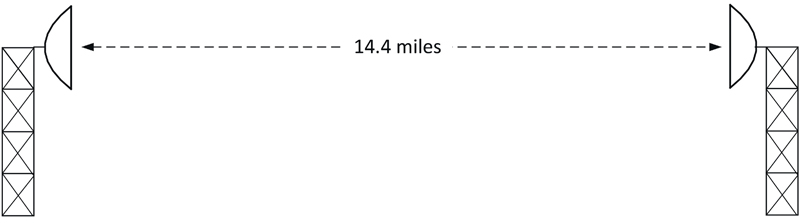
Figure 4 illustrates a hypothetical microwave path that is 14.4 miles in length. Assuming operation in the 12.7 GHz to 13.2 GHz cable television relay service (CARS) band, and a frequency of 12.7035 GHz, the free space path loss can be calculated with the formula

FSPL = 20log₁₀(f) + 20log₁₀(D) + 96.58

where FSPL is the free space path loss from the transmit antenna to the receive antenna in decibels; f is frequency in gigahertz; and D is distance in statute miles.

The free space path loss of the hypothetical point-to-point microwave path in Figure 4 is

FSPL = 20log₁₀(12.7035) + 20log₁₀(14.4) + 96.58

FSPL = 22.08 + 23.17 + 96.58

FSPL = 141.83 dB

When the free space path loss in dB and frequency in GHz are known, what has to be done to figure out a distance in statute miles? It takes a couple steps. Start with a variation of the FSPL formula:

X = FSPL – 96.58 – 20log₁₀(f)

X = 141.83 – 96.58 – 20log₁₀(12.7035)

X = 141.83 – 96.58 – 22.08

X = 23.17

Next, complete the calculation with the formula D = 10^(X/20).

D = 10^(23.17/20)

D = 10^(1.16)

D = 14.4 miles

Here the FSPL of a point-to-point microwave link has been converted to statute miles. That is, the 141.83 dB of FSPL at 12.7035 GHz is equivalent to 14.4 miles.

Wrapping up

We use the decibel to describe gain, loss, CNR, RxMER, and more. The decibel can also, in some cases and with certain caveats, be equivalent to distance or length. The latter is a different use of the dB for many, but if you hear someone describe, say, a 22 dB coax span or 7 dB fiber link, now you know what they mean.

---

 

Ron Hranac

Technical Editor, Broadband Library

rhranac@aol.com

Ron Hranac, a 54 year veteran of the cable industry, has worked on the operator and vendor side during his career. A Fellow Member of SCTE and co-founder and member of the organization’s Rocky Mountain Chapter, Ron was inducted into the Society’s Hall of Fame in 2010, is a co-recipient of the Chairman’s Award, an SCTE Member of the Year, and is a member of the Cable TV Pioneers Class of ’97. He received the Society’s Excellence in Standards award at Cable-Tec Expo 2016. He was recipient of the European Society for Broadband Professionals’ 2016 Tom Hall Award for Outstanding Services to Broadband Engineering, and was named winner of the 2017 David Hall Award for Best Presentation. He has published hundreds of articles and papers, and has been a speaker at numerous international, national, regional, and local conferences and seminars.

Images provided by author, Shutterstock